ASML-Foundation

Monday week 6

ADVANCED STATISTICS AND MACHINE LEARNING FOUNDATIONS

Introduction

What is the goal?

• Make rational inferences and decisions from data.
• Inference about unknown quantity $U$ given knowledge $K$:
  • Current data $X$
  • Other knowledge $K’$, e.g.:
    • Previous data; physical theory; expert opinion.
• Decision $D$ about action to take, given this knowledge and the utility (or loss) consequent on the results.

Why is this goal important?

• World data volume is huge:
  • Growing by 40% per year.
  • 175ZB (25TB per person) by 2025.
• Most (95%) is images and video.
  • E.g. earth observation satellite generates 1TB/day and there are thousands of them.
• Data usage is tiny:
  • ~1% is analysed.
• Automatic data analysis is crucial.

Particle physics

• One-hour’s data for LHC = One-year’s data for FB.
• 70% of all data are classified by machine learning.
• 100% charged-particle tracks vetted by NNs.
• Achieving the sensitivity of a recent LHCb search would need 10 years of data without ML.
• Determination of particle energies. - Multivariate regression, boosted decision trees.
• Detection and classification of H → γγ decays. - Boosted decision trees.
• Categorization of neutrino events in the NOvA and MicroBooNE detectors. - Computer vision using CNNs.

How to do achieve the goal?

• Remarkably, there is essentially one way to do this correctly.
• Making inferences under uncertainty:
  • Probability theory: ‘unique’ generalization of classical logic to uncertain propositions (Cox’s theorem).
• Making decisions under uncertainty:
  • Decision theory: ‘unique’ method for rational choices (von Neumann–Morgenstern utility theorem).
• Together: Bayesian statistics.

And that’s it! Easy, right? Wrong!

• Data and decisions are often very complex and high-dimensional.
  • E.g. satellite image: 200-million-dimensional vector or in a set of 10^500,000,000 elements.
    • Cf 10^80 atoms in observable universe.
  • Neural networks may have ~ 10^9 parameters.
• Constructing a probability distribution that represents enough knowledge to be useful.
  • Very difficult: most ‘images’ are just noise.
  • Perhaps not possible ‘by hand’.
• Extracting information from this distribution.
  • We need to integrate and optimize over these spaces.

Bayesian statistics in use

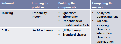
Structure

• Framework
  • Bayesian statistics: the maths of rationality
  • Cox’s theorem
  • Von Neumann-Morgenstern theorem
• Framing the problem
  • Making inferences
  • Making decisions
• Building the components
  • Ignorance
  • Information
  • Dependencies
  • Conditional models
• Computing the answer
  • The problem
  • Integration
  • Optimization

Framework

Bayesian Statistics: the mathematics of rationality

• Probability theory
  • The unique method for rational thinking
• Decision theory
  • The unique method for rational acting
• Bayesian statistics = PT + DT
• Why these ingredients?
  • Cox’s theorem
  • Von Neumann-Morgenstern theorem

Cox’s theorem

Cox’s theorem: postulates

• Concerns plausibilities $P(A

  B)$ of propositions.

  • Propositions $A, B,$ etc. meaning ‘A is true’, etc.

  • $P(A	B)$ is plausibility of A being true given that B is true.

• Axioms:
  • Comparability
    • The plausibility of a proposition is a real number (all plausibilities can be compared);
  • Rationality
    • Plausibilities should vary rationally with the variation of other plausibilities, including reducing to classical logic when all propositions are certain;
  • Consistency
    • If the plausibility of a proposition can be derived in many ways, all the results must be equal.

Cox’s theorem: unique solution

• Plausibilities satisfy:
  • Range:

    • Certain truth is represented by $P(A

      B) = 1$

    • Certain falsehood is represented by $P(A

      B) = 0$.

  • Negation:

    • $P(A

      B) + P(\neg A

      B) = 1$

      • $\neg A$ is the proposition ‘A is false’.
  • Conjunction (product rule):

    • $P(A, B

      C) = P(A

      B, C)P(B

      C)$

      • $A, B$ is the proposition ‘A and B’.

Cox’s theorem: consequences

• Bayes theorem (from product rule)
  $P(B|A, C) = \frac{P(A|B, C)P(B|C)}{P(A|C)}$

• Disjunction (sum rule)
  $P(A \vee B|C) = P(A|C) + P(B|C) - P(A, B|C)$

• Partition (extending the conversation)
  $P(A|C) = \sum_i P(A, B_i|C) = \sum_i P(A|B_i, C) P(B_i|C)$

• Often:
  $P(A|C) = \sum_i P(A|B_i) P(B_i|C)$
  Sum over all ‘paths’ from C to A.

Von Neumann-Morgenstern theorem

Von Neumann-Morgenstern theorem: postulates

• Concerns preferences ≼ between probability distributions on a set of rewards R.
  • Known as ‘gambles’.
  • $R \prec S$ means R is a worse gamble than S.
  • Decisions $d \in D$ choose between gambles. 符号有错
• Axioms:
  • Completeness
    • For two gambles R and S, either $R \prec S$, $S \prec R$, or both ($R \sim S$).
  • Transitivity
    • If $R \prec S$ and $S \prec T$, then $R \prec T$.
  • Continuity
    • If $R \prec S \prec T$, then $\exists p \in [0,1]$: $S \sim pR + (1 - p)T$.
  • Independence
    • If $R \prec S$, then $\forall T: pR + (1 - p)T \prec pS + (1 - p)T$.

Von Neumann-Morgenstern theorem: unique solution

• There exists a function $L: {R} \rightarrow \mathbb{R}$, known as the ‘loss function’, that satisfies:
  • $L(R) \geq L(S) \iff R \succ S$
  • $L(pR + (1 - p)S) = pL(R) + (1 - p)L(S)$ 符号有错
• So, to decide between gambles: Minimize the expected loss

Von Neumann-Morgenstern theorem: consequences

• Remember $L(d, u)$? How do we get there?
• Rewards (i.e. consequences of decision) are pairs $(u’, u) \in W \times W$.
  • $W$ are possible ‘states of the world’ (SoW).
  • $u$ is state of the world before decision.
  • $u’$ is state of the world after decision.
• $\tilde{L}(u’, u)$ measures how bad is the change in the SoW.
• Pick the decision $d \in \mathcal{D}$ that minimizes

  • $\langle \tilde{L} \rangle (d) = \sum_{u’} \tilde{L}(u’, u) P(u’

    u, d, K)$.

• If $u’ = f(u, d)$, then we can instead minimize

  • $\langle L \rangle (d) = \sum_{u} L(d, u) P(u

    d, K)$.

Framing the problem

Making inferences

Making inferences: set-up

• Wish to make an inference about unknown $U$:
  • Class of galaxy; location of neutrino tracks in image; energy of particle; disease diagnosis; guilt or innocence; …
• We have some knowledge $K$ already:
  • The world is 3d (or 4d or 10d); physical laws; general knowledge; previous data; expert opinion; …
• The quantity of interest for inference is what we know about $U$ given $K$:

  • $P(U

    K)$

  • We must construct this probability.
• How?!

\[S = \frac{1}{4 \pi \alpha'} \int d^2 \sigma \sqrt{|h|} h^{\alpha \beta} g_{\mu \nu} \partial_\alpha X^\mu \partial_\beta X^\nu\]

Making inferences: Bayes theorem

• We have only the product and sum rules!

• Use these to rework $P(U

  K)$ into probabilities that we can reasonably assign.

• Often $K$ splits: current data $X$ and other knowledge $K’$.
• It is frequently much easier to construct:

  • $P(X	U,K’)$: ‘causal’ data formation model.

    • E.g. image from object.

  • $P(U	K’)$: ‘theoretical’ model of $U$.

    • E.g. physics.

• Then $P(U

  X,K’) \propto P(X

  U,K’)P(U

  K’)$.

  • N.B. Normalization may be very difficult.

Making inferences: partition

• Sometimes other quantities $V$ can help:
  • Make the connection between $U, X,$ and $K$ ‘causal’.
  • Reduce dependence.
• There are several ways this can happen.
• Example:

  • $P(U

    K) \alpha \sum_V P(U

    V,K)P(V

    K)$ 有错

• Sometimes this is just an extra formal parameter.
• Sometimes it is a physical quantity.
  • Future solar exposure, rainfall, and temperature, if plant growth is being predicted from fertilizer application and other known quantities.
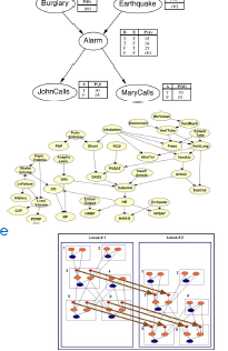
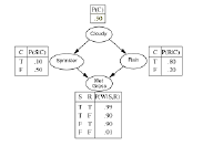
  • Alarm makes JohnCalls and MaryCalls independent.

Checkpoint

• Bayesian statistics:

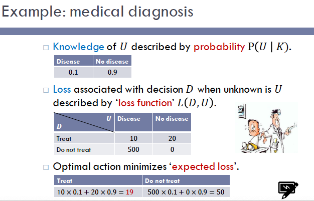
  • Probability theory is rational thinking: P(U

    K).

  • Decision theory is rational acting: L(D,U).
• Problems are how to:

  • Model and compute P(U

    K).

  • Compute and optimize E[L](D).

• Often useful to separate data X: P(U

  X,K).

  • Use Bayes’ theorem: P(U

    X,K) ∝ P(X

    U,K)P(U

    K).

• Examples:

  • Medical diagnosis: X binary, U binary: P(U

    K) and P(X

    U,K) Bernoulli.

  • Labour voting: X ∈ ℕ, U ∈ ℝ: P(U

    K) beta and P(X

    U,K) binomial.

• Often useful to introduce new unknown quantities to make the connection between U, X, and K easier to model:
  • More causal or more independence: e.g. plant growth.

Making inferences: mean of Gaussian

• We have some data $x = { x_i }_{i \in n}$.
• We will model it using a Gaussian, with unknown mean $\mu$ and variance $v$.
• We want to know about $\mu$.

  • Quantity of interest is $P(\mu

    x, K)$.

  • Note that we are not estimating $\mu$.

• Result: $\frac{(\mu - \bar{x})}{s

  x, K} \sim t(n - 1)$.

  • Familiar but quite different in meaning.

Making inferences: summaries

• Mode:
  • No measure of uncertainty.
  • Can be unrepresentative.
  • Not invariant.
• Mean:
  • No measure of uncertainty.
  • Can be unrepresentative.
• Mean and variance:
  • Can be unrepresentative.
• Credible intervals:
  • Better at summarizing uncertainty, but no estimate.
• In high dimensions, all these become difficult to compute.

Checkpoint

• Often useful to introduce new unknown quantities to make the connection between $U, X,$ and $K$ easier to model:
  • More causal or more independence: e.g. plant growth.
  • Example:
    • Introduce variance to make inference about mean.
      • Also contrast with classical t-tests.
• Summaries of distributions:
  • Pros and cons.

Making inferences: posterior predictive

• Another example of partition.
• Known $K$ is data $X = {X_i}$ and other info $K’$.
• Unknown $U$ is next piece of data $Y$.

• Quantity of interest: $P(Y

  X,K)$.

  • Given a name: ‘posterior predictive distribution’.
  • Just another special case.
• Missing information:
  • Parameters of process.
    • E.g. $P(\checkmark) = p$ and $P(\times) = 1 - p$.

Parameter estimation in integrals: plug-in estimates

• Often arises not as part of a decision, but as an approximation to an integral.
• Posterior predictive distribution is usual example.
• Leads to ‘plug-in estimates’:

  • Estimate parameter $a$ from current data $P(a

    x,K)$, giving estimate $\hat{a}$.

  • Treat it as the true value and plug into $P(y

    a,K)$ giving $P(y

    \hat{a},K)$.

Making decisions

• Once we have $P(U

  K)$, we want to use it to:

  • Tell us about $U$.
  • Make decisions.
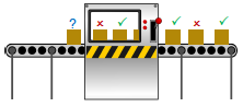
• Hypothesis testing, model selection, classification:
  • $U$ takes values in a finite set, often of two elements.
• Parameter estimation, regression:
  • $U$ takes values in an uncountable set, often $\mathbb{R}^n$.
• Unlike in classical statistics, these are just special cases of the general Bayesian statistics framework.

Making decisions: hypotheses

需修改

• Often there are two (or more) competing hypotheses/classes/models, {H_i}.
  • A classic statistical question is how to decide between them.
  • Example:
    • H_0: μ ∈ I ⊆ ℝ
    • H_1: μ ∉ I ⊆ ℝ
  • Cf term 1 data analysis and t distributions.

• As always, quantity of interest: P(H_i

  x, K).

  • We saw a two-class example of medical diagnosis.
  • Let us look at a simple approach to multi-class classification.

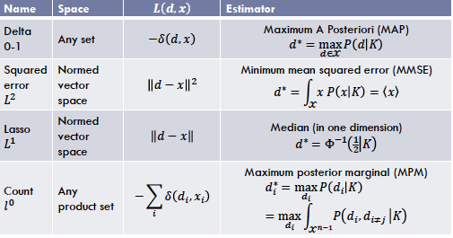
Making decisions: estimation

• Often we want to give a single-value summary of a quantity $x \in X$.
  This is called an ‘estimate’.

• The decisions $D$ are:
  • ‘Treat the value $d \in D \equiv X$ as if it were the true value’.
• Different to:
  • Distribution summary: convey information succinctly.
  • Plug-in estimate: approximate an integral.

• We need a loss function $L: X \times X \rightarrow \mathbb{R}$.
  This quantifies how bad it is to treat $d$ as the true value if it is in fact $x$.

• Should always be bespoke, but in practice…

Building the components

The problem

• We have seen:
  • The general framework for inferences and decisions.
  • Some examples.
• More generally:
  • How do we construct probability distributions that represent what we know?
• Here we will briefly describe several principles for doing this.
  • Many examples will occur in the rest of the module.

Ignorance

• What if we know nothing about a quantity U?
  • This is never true: we usually know at least a range.
  • However it may be a useful limit.
• For a finite set A, easy:
  • Ignorance means all elements are equivalent.
  • Equivalence means invariance under all permutations.

  • Invariance implies uniform distribution: $P(a) = 1/

    A

    $.

• But on a continuous set, e.g. ℝ, no distribution is invariant to all (even smooth) permutations.
  • How to define ignorance?
• Solution: Jeffreys’ prior.
  • Pullback of Fisher-Rao metric to space of parameters using the ‘likelihood’.

Convenience

• We have seen examples of conjugate priors.

• Data $D$, unknown quantity of interest $U$, probability $P(U

  D, K)$.

  • Then $P(U

    D, K) \propto P(D

    U, K)P(U

    K)$.

• If, for the given $P(D

  U, K)$ and parametric family $P(U

  K)$:

  • $P(U

    D, K)$ is in the same family, we say that $P(U

    K)$ is a conjugate prior for $P(D

    U, K)$.

• Very convenient for initial calculations.
• No longer as important with fast computers.

Information

• Sometimes we may know constraints on $P$: e.g. expectations of quantities, or averages over previous data.
• To avoid assumptions, $P$ should:
  • Maximize our ignorance
  • Be consistent with this knowledge.
• We need a measure of ignorance or uncertainty.
• Entropy $H(P)$ of a distribution $P$ on a space $X$ is the unique measure satisfying:
  • Continuity under changes in $P_i$;
  • Symmetry under permutations of $X_i$;
  • Maximality at the uniform distribution;
  • Additivity under coarsening of $X$.
• Formula:
  • $H(P) = -\sum_x P(x) \ln P(x)$ or $H(P) = -\int_X P(x) \ln \rho(x)$

Maximum entropy

• Solution to problem:
  • Maximize entropy subject to constraints.
• Examples:
  • No constraints, finite set: ⇒ uniform distribution.
  • Known mean and covariance ⇒ Gaussian.
• In general, under different constraints: any exponential family distribution:
  • $P(x) \propto \exp(-\sum_a \lambda_a f_a(x))$
  • Uniform, Gaussian, Beta, Gamma, …

Dependencies

• We may be able to characterize what one quantity tells us about another.
• This is usefully summarized in ‘graphical models’.
• Solutions:
  • Directed graphical models capture ‘causal’ relationships and joint dependencies.
  • Undirected graphical models capture spatio-temporal relationships and conditional independencies.

Directed graphical models

DGMs:

• Summarize dependency information.
• Provide a convenient ‘way to think’.
• Help to analyze models.
• Complex inferences can be expressed as graph operations, simplifying implementation.

Thus they enable:

• Construction of probability distributions that capture important dependencies.
• While keeping the models relatively simple (fewer parameters).
• Use of the resulting models in practice.

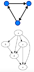
Directed acyclic graphs (DAG)

• Graph: $G = (V, E)$, where $E \subseteq V \times V$.
  • Cycle: set of edges leading back to a vertex.
  • Acyclic: containing no cycles.
• Terms:
  • Parents of $v \in V$:
    • $pa(v) = { u \in V : (u, v) \in E }$
  • Children of $v \in V$:
    • $ch(v) = { u \in V : (v, u) \in E }$
  • Ancestors of $v \in V$ and descendants of $v$ similar.

Probability distribution

• Each vertex $v \in V$ has an associated variable $x_v$.
• Probability distribution on $x = {x_v}$: \(P(x) = \prod_v P(x_v | pa(v))\)
• Advantage of structure:

  • Has $O(

    V

    A

    ^{P+1})$ parameters, where each vertex has $O(P)$ parents and takes values in $A$.

  • Cf full model with $O(

    A

    V

    )$ parameters.

Examples

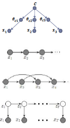
• Naïve Bayes:
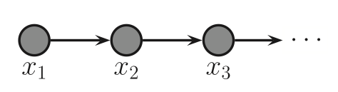
  $P(c, \theta,X) = P(c) \prod_a P(X_a|\theta_a)P(\theta_a|c)$

• Markov chain:
  $P(X) = \prod_a P(x_a|x_{a-1})$

• Second-order Markov chain:
  $P(X) = \prod_a P(x_a|x_{a-1},x_{a-2})$

• Hidden Markov models:
  $P(X,Z) = \prod_a P(X_a|Z_a)P(Z_a|Z_{a-1})$

Hierarchical models

• Simple graphical model:
  • η → θ → D

  • $P(D, θ, η) = P(D

    θ)P(θ

    η)P(η)$

• Can then calculate quantities of interest $P(U

  K)$:

  • E.g. $P(θ

    D)$ or $P(η

    D)$.

• Example: modelling cancer rates.

Conditional independence

• Minimal ancestral subgraph of set $S \in V$:
  • Smallest subgraph containing all ancestors of $S$.
• Moral graph:
  • Connect all parents of each node.
  • Drop the edge directions.
• $A \in V$ is independent of $B \in V$ given $S \in V$ iff:
  • $S$ separates $A$ and $B$ in moralized minimal ancestral subgraph of $A \cup B$.
• Markov blanket:

  • $P(v

    V \setminus v) = P(v

    N(v))$

  • $N(v) =$ neighbours of $v$ in moral graph.

Conditional models

Conditional (discriminative) models

• Sometimes it is hard to build joint models ‘by hand’:

  • $P(U

    X, K) \propto P(X

    U, K)P(U

    K) = P(X, U

    K)$

• Solution: model $P(U

  X, K)$ directly.

  1. Pick a parameterized distribution $P(U

     a)$:

     • Parameter $a$ is often the mean.
  2. Make $a$ a function of $X$:

     • $P(U

       X, f, K) = P(U

       a = f(X))$.

  3. Pick a parameterized set of functions: $f(X) \in {f_W(X)}_{W}):

     • $P(U

       X, w, K) = P(U

       a = f_W(X))$.

  4. Pick a prior for $w, P(w

     K)$.

  5. Compute $P(U

     X, K) = \int_W P(U

     X, w, K)P(w

     K)$:

     • In practice, $K$ contains previous data ${(U_i, X_i)}$.
     • Use plug-in estimates: approximate integral by estimating the parameters $w$ using MAP:

       • $P(w

         {U, X}, K) \propto P({U}

         {X}, w, K)P(w

         K) \propto P({U}

         {f_W(X)})P(w

         K)$.

• Classic examples: linear and logistic regression.

Problem:

• Hard to incorporate prior knowledge about $U$.

Solution:

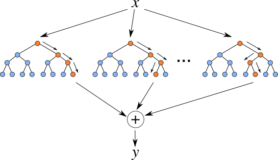
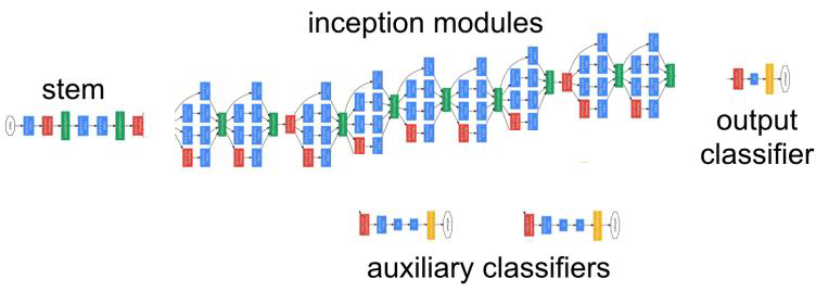
• Generic models with many parameters to capture dependencies.
• Large amounts of data needed to learn all these parameters.
• Forests, deep neural networks, …

• Can also be used for $P(X

  U, K)$.

Computing the answer

The problem

• $U$ is often lies in a very high-dimensional space.
• We need to:

  • Understand what $P(U

    K)$ tells us about $U$.

  • Calculate expectations, e.g. of the loss function.
  • Optimize to find estimates, etc.
• How to integrate and optimize over such spaces?
  • Right now, we drop a few names.
  • We will look in more detail at Monte Carlo methods.

Integration

• Analytical approximations
  • Laplace approximation and other expansions (loop,…).
• Numerical approximations

  • Variational: fit a simpler distribution to $P(U

    K)$.

    • Gaussian (‘variational Bayes’)
    • Completely factorized (mean field approximation)
    • Pairwise interactions (Bethe approximation)
      • Message-passing algorithms.
• Numerical integration
  • Monte-Carlo methods, in particular many flavours of Markov-chain Monte-Carlo.

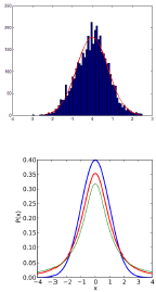
Monte Carlo approximation

• We often need to compute expectations:

  • $E[f] = \int_X f(x) P(x

    K)$

• Examples:
  • Estimation (mean, MMSE estimate).

  • Posterior predictive distribution: $f(x) = P(c

    x)$.

• Use samples ${x_i}$ from $P$ to approximate $E[f]$:
  • $\bar{f} = \frac{1}{n} \sum_i f(x_i)$
  • $E[\bar{f}] = E[f] ; \, Var[\bar{f}] = \frac{1}{n} Var[f]$.
• But need independent samples from $P$. How?
  • What does this even mean?

Sampling

• Needed: a method to sample from $U([0, 1])$.
  • These are pseudo-random number generators.
  • There is a lot of theory, but we will just assume we have one.

• Zero dimensions (discrete distributions).

• One dimension
  • Inverse transform sampling.
• Low dimensions
  • Rejection sampling.
  • Importance sampling.
• High dimensions
  • Markov Chain Monte Carlo (MCMC).
  • Low-dimensional sampling is also important for high dimensions:
    • Sampling one (or a few) variables at a time.

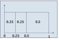
Discrete distributions

• Finite set $A$, with probabilities $P(a)$ for $a \in A$.

  • Order $A$ arbitrarily, giving $a_1, a_2, \ldots, a_{

    A

    }$.

  • Define $P_i = \sum_{j=1}^{i} P(a_i)$, with $P_0 = 0$.

  • Divide ([0,1]) into intervals ([P_{i-1}, P_i], i \in [1..

    A

    ]).

  • Let $P(x) = dx$.
    • Then $P(x \in [P_{i-1}, P_i]) = P_i - P_{i-1} = P(a_i)$.
• Algorithm
  • Sample $x$ from $U([0,1])$.
  • Return $a_i$ such that $x \in [P_{i-1}, P_i]$.

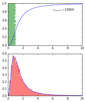
Inverse transform sampling

• We want to sample from:
  $P_Y(y) = dy \rho_Y(y)$.

• Recall:
  If $P(x) = dx$ i.e. $U([0,1])$, then under a transformation $y = \epsilon(x)$:
  $P_Y(y) = dy |(\epsilon^{-1})’(y)|$.

• Algorithm

  • Find $\epsilon^{-1}(y) = \int_0^y dz \rho_Y(z) = F_Y(y)$, the cdf of $y$.
  • Invert it to find $\epsilon$.
  • Sample ${x_i}$ from $U([0,1])$.
  • Compute ${y_i} = {\epsilon(x_i)}$.

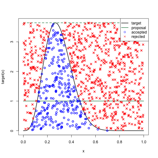
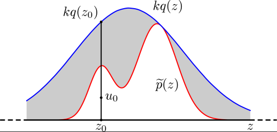
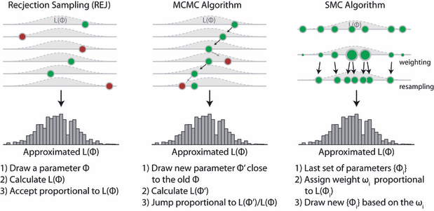
Rejection sampling

• Idea:
  • Probability is area under density.
  • Sample in 2D and throw away y value.
• Want to sample from $p = \frac{\tilde{p}}{Z_p}$, but only know $\tilde{p}$.
  • Suppose:
    • We can sample from another distribution $q$.
    • There is a $k$ such that $kq \geq \tilde{p}$.
• Algorithm
  • Sample $z_0$ from $q$.
  • Sample $u_0$ from $U([0, kq(z_0)])$.
  • If $u_0 < \tilde{p}(z_0)$, keep $x = z_0$; else reject.

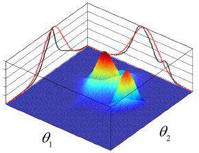
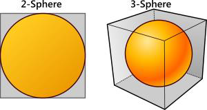
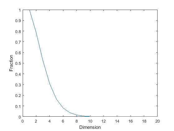
Markov Chain Monte Carlo

• In high dimensions, it is very difficult to apply rejection sampling:
  • Almost all samples are rejected.
  • E.g. hypersphere in cube.
• Abandon independent samples:
  • Generate dependent samples using Markov chains.

• Bad: more samples now needed for given variance.

• Good: very flexible, so can sample from almost any distribution.

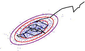
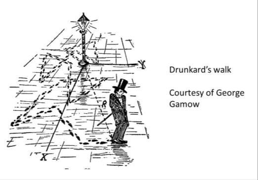
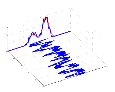
Intuition

• Probability distribution $P(x)$ on space $X$.
• Random walk in $X$ generates a series of samples.
• Ensure that the relative frequencies of values in this chain are the same as $P(x)$.
• Note that successive values are dependent.
  • Chain depends on initial point:
    • Need to eliminate burn-in.
  • Variance does not go down like $1/n$:
    • Need to estimate effective sample size.
  • Need thinning to achieve independence, but not really a good idea.

Markov chains 1

• A Markov chain is a probability distribution on variables {xi ∈ Ai}i∈ℕ.

• Markov property:

  • P(xi

    x<i) = P(xi

    xi-1).

  • Independence of past given previous value.

  • Define P(xi

    xi-1) = Ti(xi, xi-1).

    • Transition probability.
• Stationary/homogeneous:
  • Ai = ℵ
  • Ti(xi, xi-1) = T(xi, xi-1) = T(x’, x).

Markov chains 2

• Marginal probabilities related by transition probability:
  $P(x_{i+1}) = \sum_{x_i} P(x_{i+1}|x_i)P(x_i)$

• All $x$ in same space: think of evolving distribution:
  $\rho_{i+1}(x) = \sum_{x’} T(x, x’)\rho_i(x’)$

• Matrix multiplication:
  $\rho_{i+1} = T \rho_i$

• After $N$ steps:
  $\rho_{i+N} = T^N \rho_i$

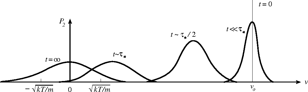
Markov chains 3

• Under certain conditions, the evolution converges to an ‘invariant’, ‘stationary, or ‘equilibrium’ distribution π that does not change:
  • Chain converges: π = (\lim_{N \to \infty} T^N \pi_0)
  • Invariant: π = Tπ
• If we sample from successive distributions in the chain, and wait long enough, our samples will become samples from π.
• So if we can construct a chain with stationary distribution the one from which we want to sample, i.e. such that π = P, we are done!
• How can we construct such Markov chains?

Gibbs sampling

• Variable $x = {x_a} \in \mathcal{A} = \prod_a A_a$. Let $

  a

  = d$.

  • Could be components, or different variables entirely.
  • Could be groups of variables.

• Sample from conditional distributions $P(x_a

  x_{\backslash a})$, updating one variable at a time:

  1. For $a = 1:d$

     1. Sample $x’_a$ from $P(x_a

        x)$

     2. Set $x_a = x’_{a}$
  2. Return $x$
  3. Go to 1
• How do we know it works?

Gibbs sampling: the good

• Only requires conditional distributions. Often:
  • Easy to find (at least unnormalized)
    • Especially for graphical models, for which conditionals are either obvious or easy to calculate.
  • Easy to sample from as low- (often one-) dimensional.
• No tuning parameters:
  • Can effectively be automated (Winbugs, Jags)

Gibbs sampling: the not-so-good

• Gibbs sampling can easily be reducible because you cannot move diagonally.
  • But if the conditional distributions are all positive, then the chain is irreducible.
• Sampling can be slow, for two reasons:
  • You cannot move diagonally.
  • Step size vs distribution size.

Metropolis-Hastings

• Splits sampling into two steps:

  • Propose a new state $x^$ according to some proposal distribution $Q(x^

    x)$.

  • Accept proposal $x’ = x^*$, or stay put $x’ = x$.
• To achieve detailed balance:
  • Accept with probability $\alpha = \min(1, R(x^*, x))$, where:
  \[R(x^*, x) = \frac{Q(x|x^*)\pi(x^*)}{Q(x^*|x)\pi(x)} = \frac{\pi(x^*)/Q(x^*|x)}{\pi(x)/Q(x|x^*)}\]
• If proposal is symmetric $R(x^, x) = \frac{\pi(x^)}{\pi(x)}$:
  • Metropolis algorithm.
• How do we know it works?

Metropolis-Hastings: the good and bad

Good

• Incredibly flexible: π can be more or less anything.
• Only ratios of π are needed, so normalization is not required.

Bad

• Choosing good proposal distributions is not always easy.
• Proposal distributions often have tuning parameters that affect acceptance probability and mixing.
  • These must usually be chosen via trial and error.

Metropolis-Hastings: common proposals

• Gaussian centred on $x$, with some (co)variance:
  $Q(x’|x) = N(x’; x, \Sigma)$.
  ‘Random walk Metropolis-Hastings’.

• Independence sampler:
  $Q(x’|x) = Q(x’)$.

• Gibbs sampler:
  $Q(x’|x) = P(x’a|x{\setminus a})\delta(x’a, x{\setminus a})$
  $P(a) = 1$.

Metropolis-Hastings: Gaussian proposals

• Small step size bad:
  • Can fail to explore space.
  • Many steps to generate a given (effective) number of samples because of high correlation.

• Large step size bad:
  • Many steps to generate a given number of samples due to large rejection probability.

• Variance adjusted using pilot runs:
  • Target 25% – 40% acceptance rate.

Metropolis-Hastings: variants

• Mixtures:
  • Pick one of a number of valid proposals at random.
• Data-driven:

  • Predictors $Q_k(x_k

    f_k(D))$ trained on data $(x,D)$ generated from model.

  • $Q(x’

    x) = p_0 Q_0(x’

    x) + \sum_k p_k Q_k(x_k

    f_k(D))$

• Adaptive:
  • Change Gaussian proposal $\Sigma$ over iterations according to empirical covariance.

• Reversible-jump (RJ-MCMC)

• Hamiltonian MCMC

MCMC: Practicalities

• Acceptance:
  • Target ~ 40% acceptance by tuning parameters via pilot runs.
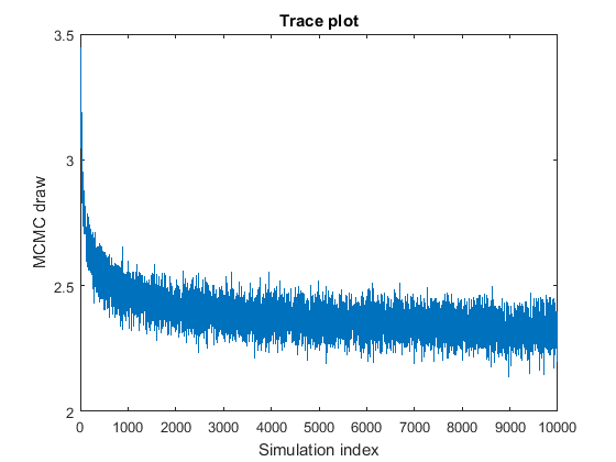
• Burn-in:
  • Eye-balling traces is still the most reliable method.
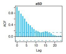
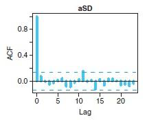
• Autocorrelation and thinning:
  • Function acf in R.
• Effective sample size:
  • Package coda in R.

Summary of methods

Recent application: MCMC GANs

• Discriminator Rejection Sampling
  • Samaneh Azadi, Catherine Olsson, Trevor Darrell, Ian Goodfellow, Augustus Odena
  • (Submitted on 16 Oct 2018 (v1), last revised 26 Feb 2019 (this version, v3))
• Metropolis-Hastings Generative Adversarial Networks
  • Ryan Turner, Jane Hung, Eric Frank, Yunus Saatci, Jason Yosinski
  • (Submitted on 28 Nov 2018 (v1), last revised 17 May 2019 (this version, v2))

Optimization

• Gradient ascent.
  • Hill climbing.
• Stochastic gradient ascent.
  • Add noise to avoid local maxima.
    • Explicitly.
    • Implicitly by training using subsets of the data.
  • Decrease noise (learning rate) slowly.
• Simulated annealing.
  • Sampling e.g. MCMC.
  • Decrease ‘temperature’ slowly.
• Message-passing algorithms.
  • Max-sum instead of sum-product.