2025-09-02-CS-E4715 - Supervised Machine Learning 1

Supervised Machine Learning 1

Introduction

Understanding machine learning

For a professional machine learning engineer / data scientist, it is useful to go beyond using machine learning tools as black boxes:

• Machine learning does not always succeed; one needs to be able to understand why and find remedies.
• Not possible to follow the scientific advances in the field without understanding the underlying principles.
• Competitive advantage: more jobs and better pay for people that have understanding of the algorithms and statistics.

Theoretical paradigms of machine learning

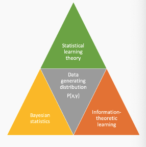
Theoretical paradigms for machine learning differ mainly on what they assume about the process generating the data:

• Statistical learning theory (focus on this course): assumes data is i.i.d from an unknown distribution $P(x)$, does not estimate the distribution (directly)
• Bayesian Statistics (focus of course CS-E5710 - Bayesian Data Analysis): assumes prior information on $P(x)$, estimates posterior probabilities
• Information theoretic learning (e.g. Minimum Description Length principle, MDL): estimates distributions, but does not assume a prior on $P(x)$

Supervised and unsupervised machine learning

• Supervised machine learning (Focus of this course)
  • training data contains inputs and outputs (=supervision)
  • goal is to predict outputs for new inputs
  • typical tasks: classification, regression, ranking
• Unsupervised machine learning (Focus of course CS-E4650 - Methods of Data Mining)
  • training data does not contain outputs
  • goal is to describe and interpret the data
  • typical tasks: clustering, association analysis, dimensionality reduction, pattern discovery

Course topics

• Part I: Theory
  • Introduction
  • Generalization error analysis & PAC learning
  • Rademacher Complexity & VC dimension
  • Model selection
• Part II: Algorithms and models
  • Linear models: perceptron, logistic regression
  • Support vector machines
  • Kernel methods
  • Boosting
  • Neural networks (MLPs)
• Part III: Additional topics
  • Feature learning, selection and sparsity
  • Multi-class classification
  • Preference learning, ranking

Supervised Machine Learning Tasks

Classification

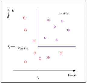
Classification deals with the problem of partitioning the data into pre-defined classes by a decision boundary or decision surface (blue line in the figure below)

• Example: In credit scoring task, a bank would like to predict is the customer should be given credit or not
• Decision can be based on available input variables: Income, Savings, Employment, Past financial history, etc.
• Output variable is a class label: low-risk (0) or high-risk (1)
• This is called binary classification since we have two classes

Multi-class classification

Multi-class classification tackles problems where there are more than two classes

• Example: hand-written character recognition
• Input: images of hand-written characters

• Output: the identity of the character (e.g. Unicode ID)

• Multi-label Classification An example can belong to multiple classes at the same time
• Extreme classification Learning with thousands to hundreds of thousands of classes

Regression

• Regression deals with output variables which are numeric

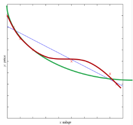
• Example: predicting the price of the car based on input variables (model, year, engine capacity, mileage)

• Linear regression: our model is a line: $f(x) = wx + w_0$

• Polynomial regression: our model is a polynomial: quadratic $f(x) = w_2x^2 + w_1x + w_0$, cubic $f(x) = w_3x^3 + w_2x^2 + w_1x + w_0$ or even higher order

• Many other non-linear regression models besides polynomials

Ranking and preference learning

• Sometimes we do not need to predict exact values but an ordered list of preferred objects is sufficient
• Example: a movie recommendation system
• Input: characteristics of movies the user has liked
• Output: an ranked list of recommended movies for the user
• Training data typically contains pairwise preferences: user x prefers movie $y_i$ over movie $y_j$

Dimensions of a supervised learning algorithm

1. Training sample: $S = {(x_i, y_i)}_{i=1}^{m}$, the training examples ((x, y) \in X \times Y) independently drawn from an identical distribution (i.i.d) (D) defined on (X \times Y), where (X) is a space of inputs and (Y) is the space of outputs.

2. Model or hypothesis $h : X \mapsto Y$ that we use to predict outputs given the inputs $x$.

3. Loss function: $L : Y \times Y \mapsto \mathbb{R}, L(\ldots) \geq 0, L(y, y’)$ is the loss incurred when predicting $y’$ when $y$ is true.

4. Optimization procedure to find the hypothesis $h$ that minimizes the loss on the training sample.

Data spaces

• The input space $X$, also called the instance space, is generally taken as an arbitrary set
  • Often $X \subset \mathbb{R}^d$, then the training inputs are vectors $\mathbf{x} \in \mathbb{R}^d$ - we use boldface font to indicate vectors
  • But they can also be non-vectorial objects (e.g. sequences, graphs, signals)
  • Often data are mapped to feature vectors in preprocessing or during learning.
• The output space $\mathcal{Y}$ containing the possible outputs or labels for the model depends on the task:
  • Binary classification: $\mathcal{Y} = {0, 1}$ or $\mathcal{Y} = {-1, +1}$
  • Multiclass classification: $\mathcal{Y} = {1, \ldots, K}$
  • Regression: $\mathcal{Y} = \mathbb{R}$
  • Multi-task/multi-label learning: $\mathcal{Y} = \mathbb{R}^d$ or $\mathcal{Y} = {-1, +1}^d$

Loss functions

• Loss function $L : \mathcal{Y} \times \mathcal{Y} \rightarrow \mathbb{R}$, measures the discrepancy $L(y, y’)$ between two outputs $y, y’ \in \mathcal{Y}$
• Used to measure an approximation of the error of the model, called the empirical risk, by computing the average of the losses on individual instances

\[\hat{R}(h) = \frac{1}{m} \sum_{i=1}^{m} L(h(x_i), y_i)\]

• Loss functions depend on the task:
  • squared loss is used in regression: $L_{sq}(y, y’) = (y’ - y)^2, \, y, y’ \in \mathbb{R}$
  • 0/1 loss is used in classification: $L_{0/1}(y, y’) = 1_{y \neq y’}$
  • Hamming loss is used in multilabel learning: $L(y, y’) = \sum_{j=1}^{d} L_{0/1}(y_j, y’_j), \, y, y’ \in {-1, +1}^d$
• Loss functions taking into account the structure of the output space or the cost of errors can also be defined

Generalization

• Our aim is to predict as well as possible the outputs of future examples, not only for training sample

• We would like to minimize the generalization error, or the (true) risk

  $R(h) = \mathbb{E}_{(x,y) \sim D} [ L(h(x),y) ]$

• Assuming future examples are independently drawn from the same distribution $D$ that generated the training examples (i.i.d assumption)
• But we do not know $D$!
• What can we say about $R(h)$ based on training examples and the hypothesis class $\mathcal{H}$ alone? Two possibilities:
  • Empirical evaluation through testing
  • Statistical learning theory (Lectures 2 and 3)

Hypothesis classes

There is a huge number of different hypothesis classes or model families in machine learning, e.g:

• Linear models such as logistic regression and perceptron
• Neural networks: compute non-linear input-output mappings through a network of simple computation units
• Kernel methods: implicitly compute non-linear mappings into high-dimensional feature spaces (e.g. SVMs)
• Ensemble methods: combine simpler models into powerful combined models (e.g. Random Forests)

Each have their different pros and cons in different dimensions (accuracy, efficiency, interpretability); No single best hypothesis class exists that would be superior to all others in all circumstances.

Optimization algorithms

The difficulty of finding the best model depends on the model family and the loss function

We are often faced with

• Non-convex optimization landscapes (e.g. neural networks) ↔ hard to find the global optimum
• NP-hard optimization problems (e.g finding a linear classifier that has the smallest empirical risk) ↔ need to use approximations and heuristics

“Big Data” with very large training sets (1 million examples and beyond) amplifies these problems

Linear regression

Example: linear regression

• Training Data: ${(x_i, y_i)}_{i=1}^m$, $(x, y) \in \mathbb{R}^d \times \mathbb{R}$
• Loss function: squared loss $L_{sq}(y, y’) = (y - y’)^2$
• Hypothesis class: hyperplanes $h(\mathbf{x}) = \sum_{j=1}^d w_j x_j + w_0$
• Model: $y = h(\mathbf{x}) + \epsilon$, where $\epsilon$ is random noise corrupting the output. We assume zero-mean normal distributed noise: $\epsilon \sim \mathcal{N}(0, \sigma^2)$, with unknown $\sigma$
• Optimization: essentially, inverting a matrix (low polynomial time complexity)

Optimization problem

\[\begin{aligned} & \text{minimize} \quad \sum_{i=1}^m \left(y_i - \left(\sum_{j=1}^d w_j x_{ij} + w_0\right)\right)^2 \\ & w.r.t. \ w_j, j = 0, \ldots, d \end{aligned}\]

Write this in matrix form:

\[\begin{aligned} & \text{minimize} \quad (\mathbf{y} - \mathbf{X}\mathbf{w})^T (\mathbf{y} - \mathbf{X}\mathbf{w}) \\ & w.r.t. \ \mathbf{w} \in \mathbb{R}^{d+1} \end{aligned}\]

where

\[\mathbf{X} = \begin{bmatrix} 1 & \mathbf{x}_1 \\ \vdots & \vdots \\ 1 & \mathbf{x}_i \\ \vdots & \vdots \\ 1 & \mathbf{x}_m \end{bmatrix}, \ \mathbf{w} = \begin{bmatrix} w_0 \\ w_1 \\ \vdots \\ w_d \end{bmatrix}, \ \mathbf{y} = \begin{bmatrix} y_1 \\ \vdots \\ y_i \\ \vdots \\ y_m \end{bmatrix}\]

Minimum of

\[\textit{minimize} \quad (\mathbf{y} - \mathbf{X}\mathbf{w})^T (\mathbf{y} - \mathbf{X}\mathbf{w}) \\ w.r.t.\mathbf{w} \in \mathbb{R}^{d+1}\]

is attained when the derivatives w.r.t w go to zero

\[\frac{\partial}{\partial \mathbf{w}} (\mathbf{y} - \mathbf{X}\mathbf{w})^T (\mathbf{y} - \mathbf{X}\mathbf{w}) \\ = \frac{\partial}{\partial \mathbf{w}} \mathbf{y}^T \mathbf{y} - \frac{\partial}{\partial \mathbf{w}} 2 (\mathbf{X}\mathbf{w})^T \mathbf{y} + \frac{\partial}{\partial \mathbf{w}} (\mathbf{X}\mathbf{w})^T \mathbf{X} \mathbf{w} \\ = -2 \mathbf{X}^T \mathbf{y} + 2 (\mathbf{X}^T \mathbf{X}) \mathbf{w} = 0\]

This gives us a set of linear equations $\mathbf{X}^T \mathbf{y} = (\mathbf{X}^T \mathbf{X}) \mathbf{w}$ that can be solved by inverting $\mathbf{X}^T \mathbf{X}$:

\[\mathbf{w} = (\mathbf{X}^T \mathbf{X})^{-1} \mathbf{X}^T \mathbf{y}\]

if $\mathbf{X}^T \mathbf{X}$ invertible, and by computing a pseudo-inverse, otherwise

Binary classification

Binary classification

• Goal: learn a class $C$, $C(\mathbf{x}) = 1$ for members of the class, $C(\mathbf{x}) = 0$ for others
• Example: decide if car is a family car $(C(\mathbf{x}) = 1)$ or not $(C(\mathbf{x}) = 0)$
• We have a training set of labeled examples
  • positive examples of family cars
  • negative examples of other than family cars
• Assume two relevant input variables have been picked by a human expert: price and engine power

Data representation

• The inputs are 2D vectors
  \(\mathbf{x} = \begin{bmatrix} x_1 \\ x_2 \end{bmatrix} \in \mathbb{R}^2, \text{ where } x_1 \text{ is the price and } x_2 \text{ is the engine power}\)
• The label is a binary variable
  \(y = \begin{cases} 1 & \text{if } \mathbf{x} \text{ is a family car} \\ 0 & \text{if } \mathbf{x} \text{ is not a family car} \end{cases}\)
• Training sample $ S = {(\mathbf{x}i, y_i)}{i=1}^m $ consists of training examples, pairs $(\mathbf{x}, y)$
• The labels are assumed to usually satisfy $ y_i = C(\mathbf{x}_i) $, but may not always do e.g. due to intrinsic noise in the data

Hypothesis class

• We choose as the hypothesis class
  $\mathcal{H} = { h : X \mapsto {0, 1} }$ the set of axis parallel rectangles in $\mathbb{R}^2$
  \(h(\mathbf{x}) = (p_1 \leq x_1 \leq p_2) AND (e_1 \leq x_2 \leq e_2)\)

• The classifier will predict a ”family car” if both price and engine power are within their respective ranges
• The learning algorithm chooses a $h \in \mathcal{H}$ by assigning values to the parameters $(p_1, p_2, e_1, e_2)$ so that $h$ approximates $C$ as closely as possible

However, we do not know $C$, so cannot measure exactly how close $h$ is to $C$!

Version space

If a hypothesis correctly classifies all training examples we call it a consistent hypothesis

• Version space: the set of all consistent hypotheses of the hypothesis class
• Most general hypothesis G: cannot be expanded without including negative training examples
• Most specific hypothesis S: cannot be made smaller without excluding positive training points

Margin

• Intuitively, the “safest” hypothesis to choose from the version space is the one that is furthers from the positive and negative training examples
• Margin is the minimum distance between the decision boundary and a training point

The principle of choosing the hypothesis with a maximum margin is used, e.g. in Support Vector Machines

Model evaluation

Zero-one loss

• The most commonly used loss function for classification is the zero-one loss: $L_{0/1}(y, y’) = \mathbf{1}_{y \neq y’}$ where $\mathbf{1}_A$ is the indicator function:

\[\mathbf{1}_A = \begin{cases} 1 & \text{if } A \text{ is true} \\ 0 & \text{otherwise} \end{cases}\]

• However, zero-one loss is not a good metric when the class distributions are imbalanced
  • consider a binary problem with 9990 examples in class 0 and 10 examples in class 1
  • if model predicts everything to be class 0, accuracy is $ \frac{9990}{10000} = 99.9\% $ which is misleading
• Class-dependent misclassification costs are another weakness:
  • consider we are dealing with a rare but fatal disease, the cost of failing to diagnose the disease of a sick person is much higher than the cost of sending a healthy person to more tests

Confusion matrix

In binary classification, the zero-one loss is composed of

• False positives
  ${x_i : h(x_i) = 1 \text{ and } y_i = 0}$ and
• False negatives
  ${x_i : h(x_i) = 0 \text{ and } y_i = 1}$
• Generally
  • making the hypothesis more specific leads to increased false negative rate and decreased false positive rate (here: smaller rectangle)
  • making the hypothesis more general (here: larger rectangle) does the opposite
• Consider all four possible combinations of the predicted label (0 or 1) and the actual label (0 or 1)

• The counts of examples in the four combinations can be compactly represented in a confusion matrix

• True Positives: $m_{TP} =

  { \mathbf{x}_i : h(\mathbf{x}_i) = 1 \text{ and } y_i = 1}

  $

• True Negatives: $m_{TN} =

  { \mathbf{x}_i : h(\mathbf{x}_i) = 0 \text{ and } y_i = 0}

  $

• False Positives: $m_{FP} =

  { \mathbf{x}_i : h(\mathbf{x}_i) = 1 \text{ and } y_i = 0}

  $

• False Negatives: $m_{FN} =

  { \mathbf{x}_i : h(\mathbf{x}_i) = 0 \text{ and } y_i = 1}

  $

From the confusion matrix, many evaluation metrics besides can be computed

• Empirical risk (zero-one loss as the loss function):
  \(\hat{R}(h) = \frac{1}{m} \left(m_{FP} + m_{FN}\right)\)
• Precision or Positive Predictive Value:
  \(Prec(h) = \frac{m_{TP}}{m_{TP}+m_{FP}}\)
• Recall or Sensitivity:
  \(Rec(h) = \frac{m_{TP}}{m_{TP}+m_{FN}}\)
• F1 score:
  \(F_1(h) = 2 \frac{Prec(h) \cdot Rec(h)}{Prec(h) + Rec(h)} = \frac{2 m_{TP}}{2 m_{TP} + m_{FP} + m_{FN}}\)

And many others see e.g.
https://en.wikipedia.org/wiki/Confusion_matrix

Receiver Operating Characteristics(ROC)

• ROC curves summarize the trade-off between the true positive rate and false positive rate for a predictive model using different probability thresholds.

• Consider a system which returns an estimate of the class probability $\hat{P}(y

  x)$ or a any score that correlates with it.

• We may choose a threshold $\theta$ and make a classification rule:

\[h(\mathbf{x}) = \begin{cases} 1 & \text{if } \hat{P}(y|x) \geq \theta \\ 0 & \text{otherwise} \end{cases}\]

• For high values of $\theta$ prediction will be 0 for large fraction of the data (and there are likely more false negatives), for low values of $\theta$ prediction will be 1 for a large fraction of data (and there are likely more false positives)

• Taking into account all possible values $\theta$ we can plot the resulting ROC curve, x-coordinate: False positive rate $FPR = \frac{m_{FP}}{m}$, y-coordinate: True positive rate $TPR = \frac{m_{TP}}{m}$
• The higher the ROC curve goes, the better the algorithm or model (higher TP rate for the same FP rate)
• If two ROC curves cross it means neither model/algorithm is globally better
• The curve is sometimes summarized into a single number, the area under the curve (AUC or AUROC)

Model evaluation by testing

• How to estimate the model’s ability to generalize on future data
• We can compute an approximation of the true risk by computing the empirical risk on a independent test sample:

\[R_{test}(h) = \sum_{(x_i, y_i) \in S_{test}}^{m} L(h(x_i), y_i),\]

• The expectation of $R_{test}(h)$ is the true risk $R(h)$
• Why not just use the training sample?
  • Empirical risk $\hat{R}(h)$ on the training sample is generally lower than the true risk, thus we would get overly optimistic results
  • The more complex the model the lower empirical risk on training data: we would select overly complex models
  • ”Learning $\neq$ Fitting”

Summary

• Supervised machine learning is concerned about building models that efficiently and accurately predict output variables from input variables.
• Many different supervised learning tasks: classification, regression, ranking
• Loss functions are used to measure how accurately the model predicts the output
• The ultimate interest in machine learning is generalization: the models’ ability to generalize to new data