CV Lecture 3

Why and How do we characterise an image

• The holy grail of computer vision is to develop algorithms that extract sufficient information from an image
• This would let us transmit an image between Internet nodes, even at great distances, and then reconstruct it efficiently
• So far, we have seen examples of
  • Edges: modelled as discontinuities in the image space
  • Colour: a number of colour spaces exist

Feature detection • Finding points of interest

Feature description • Finding ways to describe the surroundings of these points

Extracting features from images

• Feature extraction is an important part of many image processing methods
• Applications include image panorama stitching, matching and robotics
• The ideal feature extraction method must be robust to changes in illumination, rotation, scale, noise and other transformations
• It also must be sufficiently fast to be of use in real-time applications

Why do we need interest points?

• Interest points are a fundamental concept in computer vision
• They enable efficient and effective analysis of visual data
• They facilitate tasks such as object recognition, image matching, and tracking of targets for various applications

How do we use interest points?

• Localisation and Matching
  • provide a way to identify specific regions of interest, making it possible to align and compare images for tasks like object recognition, image stitching, and tracking
• Feature descriptors
  • descriptors encode local image information around the found interest points, providing a compact representation of the local image structure
  • This is valuable for matching and recognizing objects in different images

How do we use interest points (IP)?

• Object recognition and tracking
  • IP help in identifying and following objects in video sequences, enabling applications such as surveillance, robotics, and augmented reality
• Efficient image registration
  • IP are used for image registration, aligning two or more images to ensure they are in the same coordinate system
  • This is essential for applications like medical image analysis, where aligning images from different modalities or time points is common

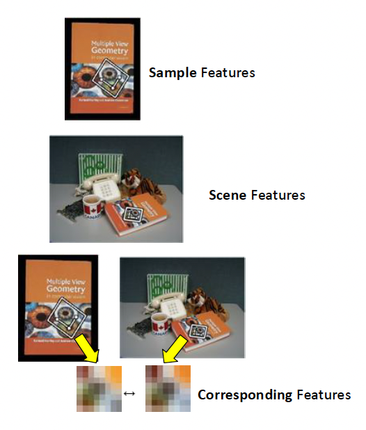
Example

• Identify generic features within a sample target
• Identify generic features within a query scene image

• If a subset of scene features and sample features match
  → Sample Target is Detected
  (in a given position and orientation/pose)

• Generalize to object classes {people, car ….}

Main characteristics of interest points

• Scale and Rotation Invariance
  • robust in handling variations in object size and orientation, allowing for more reliable recognition across different scenes and viewpoints
• Robustness to illumination changes and noise
  • IP must be suitable for applications where lighting conditions may vary
  • This is important for tasks such as object recognition in different lighting environments
  • IP must deal with noisy images
• Computational efficiency
  • IP must allow for more efficient processing of visual information. This is particularly important in real-time applications where computational resources are limited.
• Reducing data dimensionality
  • IP must reduce the dimensionality of an image, capturing only the most relevant information.
  • This is important for efficiency in terms of both computation and memory, particularly in real-time applications and systems with limited resources.

Why local features?

• Locality
  • features are local, so robust to occlusion and clutter
• Distinctiveness
  • can be employed to disambiguate in a large database
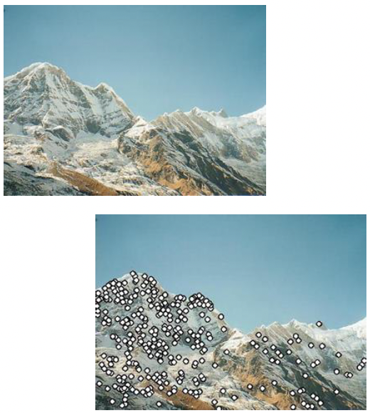
• Quantity
  • hundreds or thousands in a single image
• Efficiency
  • real-time performance is achievable
• Generality
  • exploit different types of features in different situations

Interest point detectors

• Many have been proposed in research, for different applications
• Corner detectors
• Scale-Invariant Feature Transform (SIFT)
• Speeded Up Robust Feature (SURF)
• Orientated FAST and Robust BRIEF (ORB).

Corner detector

• To detect the corners of objects in an image, one can start by detecting edges then determining where two edges meet.

• In the distant past (the long gone 1980s) two main corner detectors led the pack:

  • the Moravec detector [Moravec 1980],
  • the Harris detector [Harris & Stephens 1988].

Moravec corner detector

• The principle of this detector is to observe if a sub-image changes significantly, when we move around one pixel in all directions from a given pixel position. If this is the case, then the considered pixel is a corner.

What does this mean mathematically?

• Mathematically, the change is characterized for each pixel $(m,n)$ of an image by

\[E_{m,n}(\Delta x,\Delta y) = \sum_{u,v} w_{m,n}(u,v) [I(u + \Delta x, v + \Delta y) - I(u,v)]^2\]

• The equation represents the difference between the sub-images for an offset $(\Delta x,\Delta y)$
• $\Delta x$ and $\Delta y$ are the offsets in the 4 directions ${(1,0), (1,1), (0,1), (-1,1)}$

\[E_{m,n}(\Delta x,\Delta y) = \sum_{u,v} w_{m,n}(u,v) [I(u + \Delta x, v + \Delta y) - I(u,v)]^2\]

• For each pixel, for the four directions (up, down, left and right) the minimum is kept and denoted $F_{m,n}$ • Finally, the detected corners correspond to the local maxima of $F_{m,n}$, that is, at pixels $(m,n)$ where the smallest value of $E_{m,n}(\Delta x,\Delta y)$ is large, in practice above a given threshold • $w_{m,n}$ is a rectangular window around pixel (m,n) • $[I(u + \Delta x, v + \Delta y) - I(u,v)]$ is the difference between the sub-image I(u,v) and the offset patch

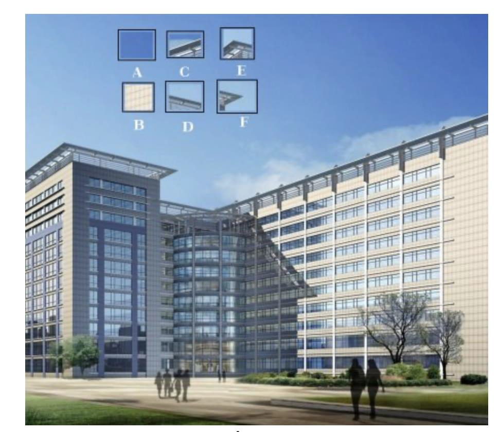
Intuition

Excerpt from an article by Harris

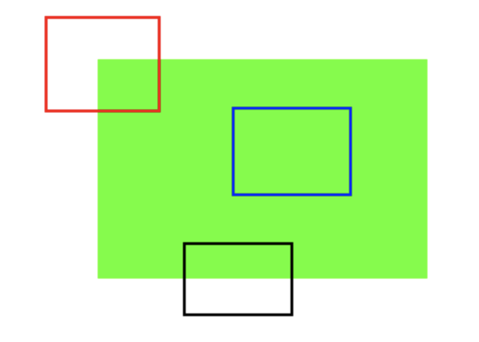
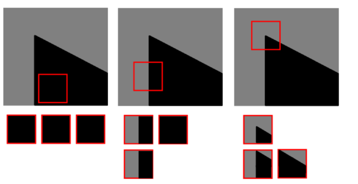
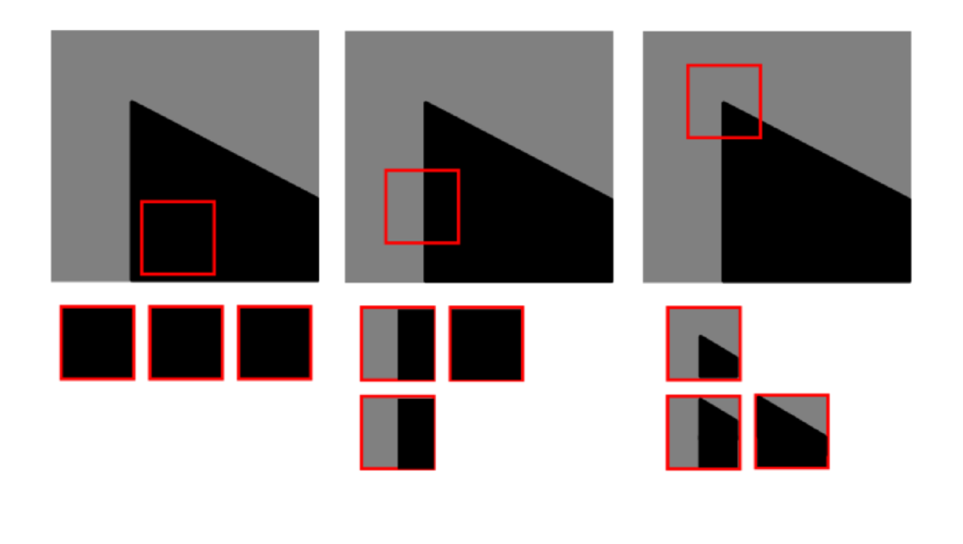
A. If the windowed image patch is flat (i.e. approximately constant in intensity), then all shifts will result in only a small change;

B. If the window straddles an edge, then a shift along the edge will result in a small change, but a shift perpendicular to the edge will result in a large change;

C. If the windowed patch is a corner or isolated point, then all shifts will result in a large change. A corner can thus be detected by finding when the minimum change produced by any of the shifts is large.

import cv2
import numpy as np
import matplotlib.pyplot as plt
import requests
from PIL import Image
from io import BytesIO

def moravec_corner_detection(image, window_size=3, threshold=100):
    rows, cols = image.shape
    offset = window_size // 2
    corner_response = np.zeros(image.shape, dtype=np.float32)

    for y in range(offset, rows - offset):
        for x in range(offset, cols - offset):
            min_ssd = float('inf')
            for shift_x, shift_y in [(1, 0), (0, 1), (1, 1), (1, -1)]:
                ssd = 0.0
                for dy in range(-offset, offset + 1):
                    for dx in range(-offset, offset + 1):
                        if (0 <= y + dy < rows) and (0 <= x + dx < cols) and \
                           (0 <= y + dy + shift_y < rows) and (0 <= x + dx + shift_x < cols):
                            diff = image[y + dy, x + dx] - image[y + dy + shift_y, x + dx + shift_x]
                            ssd += diff ** 2

                min_ssd = min(min_ssd, ssd)
            corner_response[y, x] = min_ssd

    corner_response[corner_response < threshold] = 0
    corners = np.argwhere(corner_response > 0)
    corners = [(x, y) for y, x in corners]
    return corners

Limitations of Moravec operator

• Limitations:
  • w is a binary window and therefore the detector considers all pixels in the window with the same weight
  • High noise leads to false corner detection
  • Only four directions are considered
  • The detector remains very sensitive to edges because only the minimum of is considered

Harris corner detector

• To avoid a noisy response, the rectangular window of the Moravec detector is replaced by a Gaussian window in the expression of $E_{m,n}(x,y)$.

• To extend the Moravec detector to all directions, not limited to the initial four directions, a Taylor series expansion is performed on the shifted sub-image $I(u + x, v + y)$:

\[I(u + x, v + y) \approx I(u, v) + x \partial_x I(u, v) + y \partial_y I(u, v)\]

Harris corner detector

• The approximation of the previous slide leads to changes in the value of $E_{m,n}(x,y)$

  \[E_{m,n}(x,y) \approx \sum_{u,v} w_{m,n}(u,v) [x\partial_xI(u,v) + y\partial_yI(u,v)]^2\]

• The above expression can then be rewritten in vector-matrix format as follow

  \[E_{m,n}(x,y) \approx (x \; y) M \begin{pmatrix} x \\ y \end{pmatrix}\]

Where, $M$ is the second moment matrix (also called the structure tensor)

\[M = \sum_{u,v} w_{m,n}(u,v) \begin{pmatrix} (\partial_xI)^2 & \partial_xI \partial_yI \\ \partial_xI \partial_yI & (\partial_yI)^2 \end{pmatrix}\]

Harris solves Moravec’s problems

• Finally, the last limit of the Moravec detector can be avoided by considering a new measure of the presence of a corner
• $M$ eigenvalues are used to determine the presence of a corner
• More information about the intensity change in the window can be obtained by analysing the eigenvalues and of the matrix

Alternative to eigenvalues

• Indeed, the presence of a corner is attested if the derivatives of are very large, then has large coefficients, and its eigenvalues are also very large.

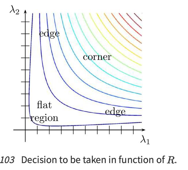
• The calculation of the eigenvalues of can be difficult, so an alternative is to calculate the corner response $R$

  \[R = \det(M) - k({trace}(M))^2 = \lambda_1\lambda_2 - k(\lambda_1 + \lambda_2)^2\]
• Thus, the values of $R$ are low in a flat region, negative on an edge, and positive on a corner.

Shi and Tomasi corner detector

• It appeared in a paper published in 1994, developed for a tracking algorithm
• It proposes a modification of the corner detector of Harris

\[R = \lambda_1 \lambda_2 - k(\lambda_1 + \lambda_2)^2\]

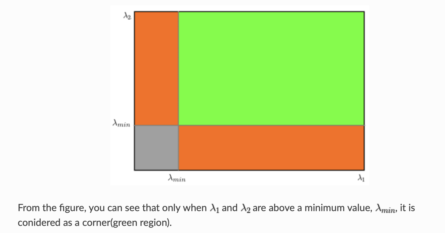
Instead of this, Shi-Tomasi proposed:

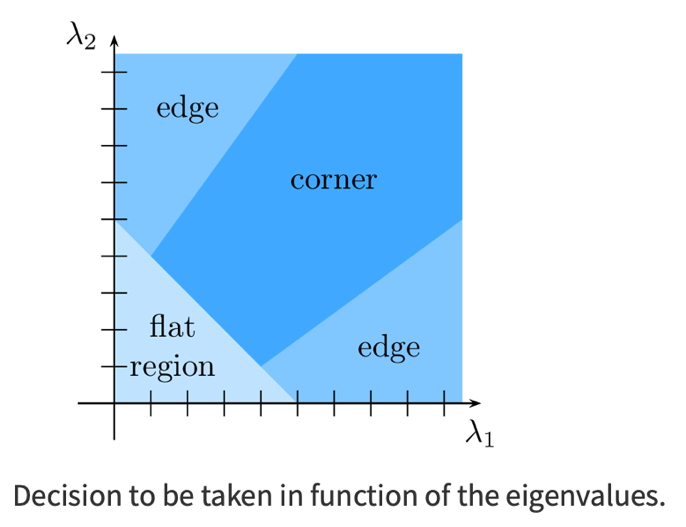
\[R = \min(\lambda_1, \lambda_2)\]

From the figure, you can see that only when $\lambda_1$ and $\lambda_2$ are above a minimum value, $\lambda_{min}$, it is considered as a corner (green region).

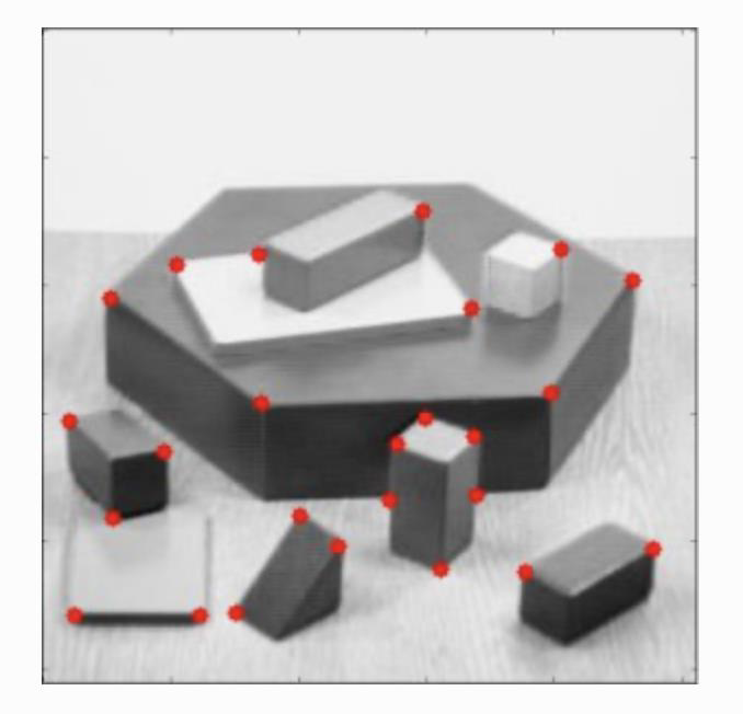
Python code

• The code using OpenCV is simple to use

import numpy as np
import cv2
from matplotlib import pyplot as plt

img = cv2.imread('simple.jpg')
gray = cv2.cvtColor(img, cv2.COLOR_BGR2GRAY)

corners = cv2.goodFeaturesToTrack(gray, 25, 0.01, 10)
corners = np.int0(corners)

for i in corners:
    x, y = i.ravel()
    cv2.circle(img, (x, y), 3, 255, -1)

plt.imshow(img), plt.show()

That was the past …

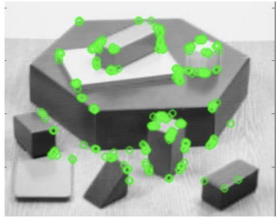
Interest points so far

• So far, with simple or slightly more complex methods, we developed ways to detect corners, also called interest points
• We want a bit more than that, in fact we want ways to find the points of interest, but also create description for them
• We will then be able to develop algorithms that perform more efficiently at the task at hand, for instance matching characteristics between images

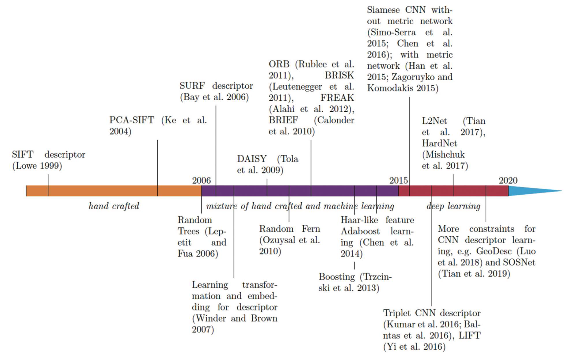
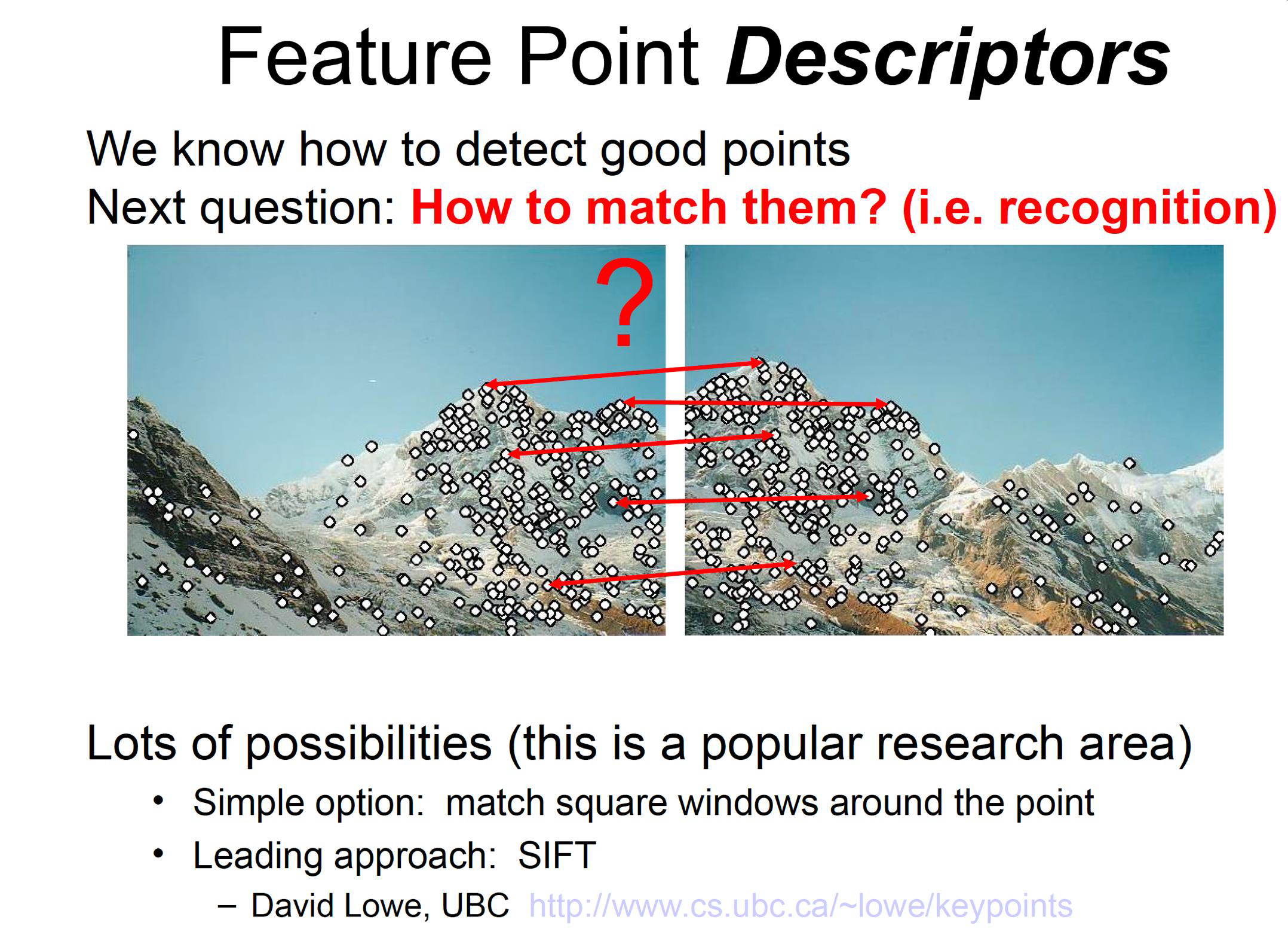
Scale-Invariant Feature Transform (SIFT)

• SIFT was devised in 2004 by David Lowe at the University of British Columbia
• He solved the problem of scale variance for feature extraction
• SIFT can be broken down into two parts
  • key-point detection
  • key-point descriptor extraction

Key point detection

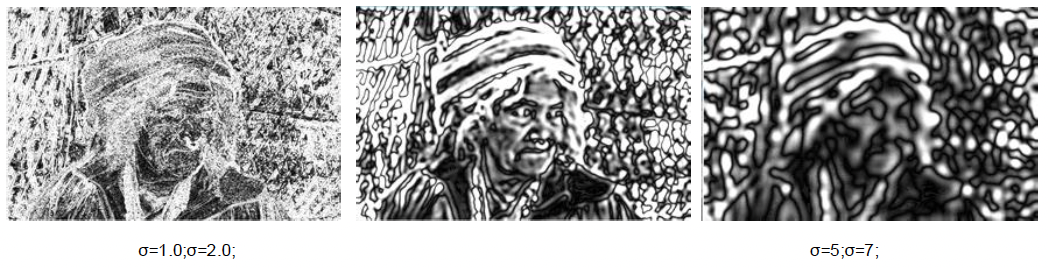
• It is implemented by approximating the Laplacian of Gaussians
• It solves the scale variance problem, but it is expensive to compute; it uses the Difference of Gaussian (DoG)
• DoG is used to search for local extrema in a 3x3x3 neighbourhood to be identified as key-points, where the third dimension is spatial scale

LoG and DoG

\[LoG(x, y) = -\frac{1}{\pi \sigma^4} \left( 1 - \frac{x^2 + y^2}{2\sigma^2} \right) e^{-\frac{x^2+y^2}{2\sigma^2}}\]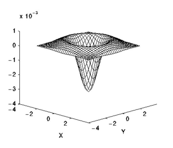

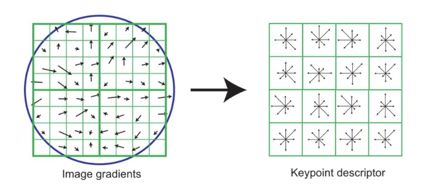
Key Point descriptor

• An orientation is assigned to each key point.
• This is done by extracting the neighbourhood around the key point and creating an orientation histogram
  • Remember the histogram of gradients (HOG)?
• The peak of the histogram is used as the orientation.
• Any other peak above 80% is also considered for the calculation
• To generate the descriptor, a 16x16 neighbourhood around a key point is taken and divided into 4x4 cells
• An orientation histogram is calculated for each cell and the combined histograms are concatenated into a 128 dimensions feature descriptor
• This is really very similar to how HOG works

From gradients to the descriptor

Scale Invariant Feature Transform (SIFT)

1. Compute Difference of Gaussian (DoG)
   (i.e. same image, two diff. levels of Gauss. filtering, subtract one from other)

SIFT - Feature Point Filtering

1. Find the local maximal pixels in space and scale
   (i.e. over σ, max of 3x3 neighbourhood)

2. Interpolate intermediate values
   (i.e. to get point location accurately)

3. Discard feature points in regions of low-contrast

1. Compute Hessian matrix, H.

   Compute ratio R:

   \[R = \frac{(trace(H))^2}{determinant(H)}\]

   (equivalent to ratio of eigenvalues of H)

   Reject if $R > \frac{(r^{th} + 1)}{r^{th}}$ $(r^{th} = 10)$

   Removes poorly localised points (varying “along/on edge” etc.)

   \[H_f = \begin{bmatrix} \frac{\partial^2 f}{\partial x_1^2} & \frac{\partial^2 f}{\partial x_1 \partial x_2} & \cdots & \frac{\partial^2 f}{\partial x_1 \partial x_n} \\ \frac{\partial^2 f}{\partial x_2 \partial x_1} & \frac{\partial^2 f}{\partial x_2^2} & \cdots & \frac{\partial^2 f}{\partial x_2 \partial x_n} \\ \vdots & \vdots & \ddots & \vdots \\ \frac{\partial^2 f}{\partial x_n \partial x_1} & \frac{\partial^2 f}{\partial x_n \partial x_2} & \cdots & \frac{\partial^2 f}{\partial x_n^2} \end{bmatrix}\]

   That is, the entry of the $i$-th row and the $j$-th column is

   \[(\mathbf H_f)_{i,j} = \frac{\partial^2 f}{\partial x_i \partial x_j}.\]

Tracking SIFT points

Speeded-up Robust feature (SURF)

• SURF was created as an improvement on SIFT in 2006, aimed at increasing the speed of the algorithm

SURF simplifies SIFT

• In the early 2000, SIFT demonstrated a remarkable performance, compared to existing descriptors
• The SURF descriptor is based on similar properties
• SIFT complexity is simplified and based on two main steps
  • The first step consists of fixing a reproducible orientation based on information from a circular region around the interest point
  • A square region is constructed and aligned to the selected orientation
  • The SURF descriptor is then extracted from it

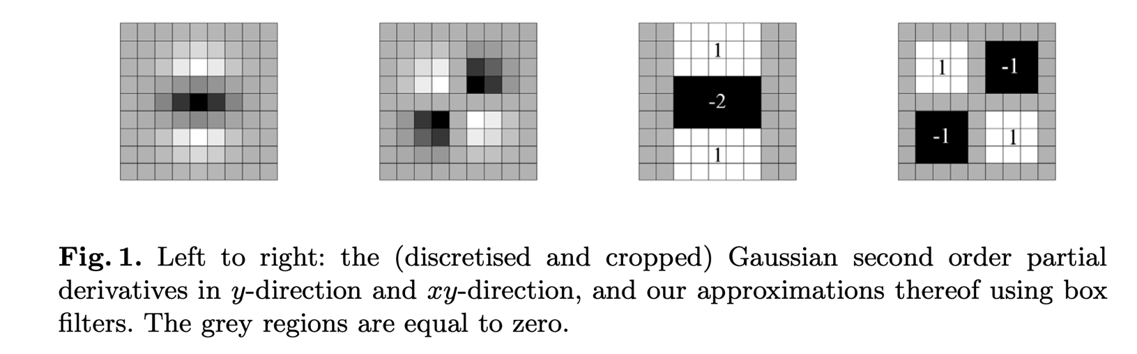
Box filters

• Rather than using Difference of Gaussian to approximate LoG, SURF utilises Box Filters
• The benefit is that box filters can be easily calculated and calculations for different scales can be done simultaneously
• The 9 × 9 box filters in Fig. 1 are approximations for Gaussian second order
• derivatives with σ = 1.2 and represent our lowest scale (i.e. highest spatial resolution)

SURF descriptor

• To extract the features of a key point, a 20s x 20s neighbourhood is extracted and divided into 4x4 cells
• Wavelet responses in x and y are extracted from each cell and responses from each cell are concatenated to form a 64 dimension feature descriptor

We want the interest point to be rotation invariant

• The Haar wavelet is used in x and y directions, in a circular neighbourhood of radius 6s, where s is the scale at which the point was detected
• The sum of the responses in a sliding scanning area is used to determine the orientation

Haar wavelet

It is a sequence of rescaled “square-shaped” functions which together form a wavelet family or basis.

The Haar wavelet’s mother wavelet function $\psi(t)$ can be described as

\[\psi(t) = \begin{cases} 1 & 0 \leq t < \frac{1}{2}, \\ -1 & \frac{1}{2} \leq t < 1, \\ 0 & \text{otherwise}. \end{cases}\]

Its scaling function $\varphi(t)$ can be described as

\[\varphi(t) = \begin{cases} 1 & 0 \leq t < 1, \\ 0 & \text{otherwise}. \end{cases}\]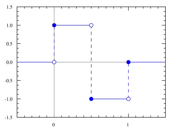

Examples for the SURF detector

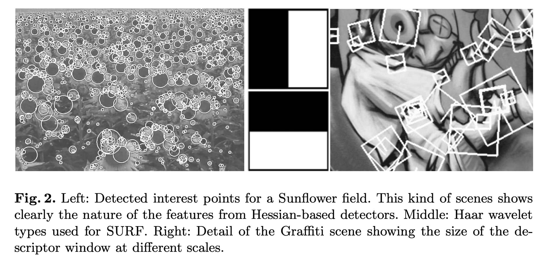
Descriptor components (step 1)

• first step consists of constructing a square region centered around the interest point, and oriented along the orientation selected in the previous section
• The region is split up regularly into smaller 4 × 4 square sub-regions
  • This keeps important spatial information
• For each sub-region, we compute a few simple features at 5×5 regularly spaced sample points

Descriptor components (step 2)

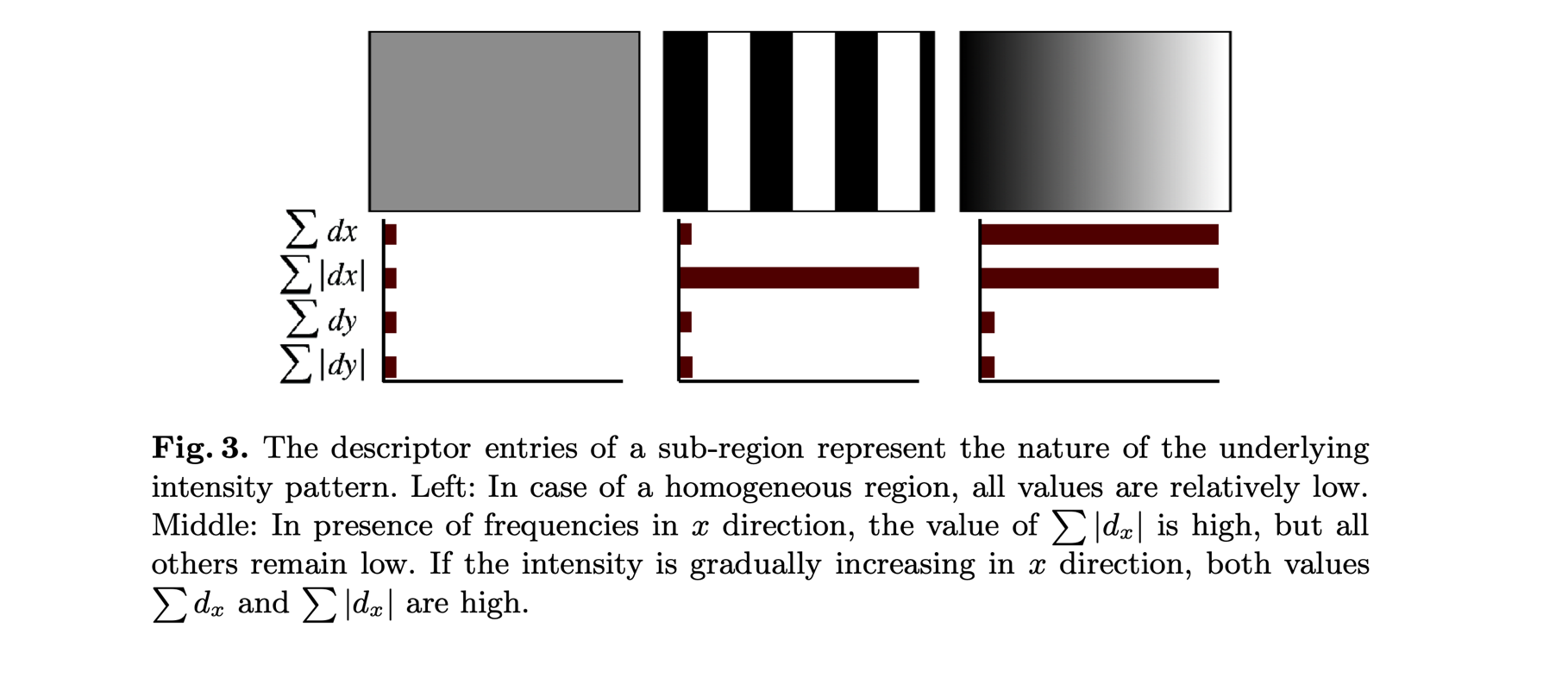
Then, the wavelet responses $d_x$ and $d_y$ are summed up over each subregion and form a first set of entries to the feature vector. In order to bring in information about the polarity of the intensity changes, we also extract the sum of the absolute values of the responses, $

d_x

$ and $

d_y

$. Hence, each sub-region has a four-dimensional descriptor vector $\mathbf{v} = \left( \sum d_x, \sum d_y, \sum

d_x

, \sum

d_y

\right)$. This results in a descriptor vector for all $4 \times 4$ sub-regions of length 64. The wavelet responses are invariant to a bias in illumination (offset). Invariance to contrast (a scale factor) is achieved by turning the descriptor into a unit vector.

• Fig. 3 shows the properties of the descriptor for three distinctively different image intensity patterns within a subregion • One can imagine combinations of such local intensity patterns, resulting in a distinctive descriptor

Oriented FAST and Rotated BRIEF (ORB)

• Developed at OpenCV labs by Ethan Rublee, Vincent Rabaud, Kurt Konolige, and Gary R. Bradski in 2011
• It is an efficient and viable alternative to SIFT and SURF
• SIFT and SURF are patented while ORB is open source
• ORB performs as well as SIFT on the task of feature detection (and is better than SURF), while being almost two orders of magnitude faster
• ORB builds on the well-known FAST key point detector and the BRIEF descriptor

ORB Main Features

• The addition of a fast and accurate orientation component to FAST
• The efficient computation of oriented BRIEF features
• Analysis of variance and correlation of oriented BRIEF features
• A learning method for decorrelating BRIEF features under rotational invariance, leading to better performance in nearest neighbour applications

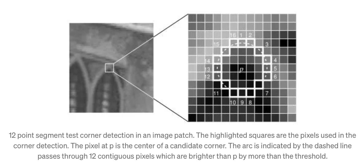
FAST

• Select a pixel p in the image which is to be identified as an interest point or not. Let its intensity be $I_p$.
• Select appropriate threshold value $t$.
• Consider a circle of 16 pixels around the pixel under test. (This is a Bresenham circle of radius 3.)
• Now the pixel p is a corner if there exists a set of $n$ contiguous pixels in the circle (of 16 pixels) which are all brighter than $I_p + t$, or all darker than $I_p - t$. (The authors have used $n = 12$ in the first version of the algorithm.)

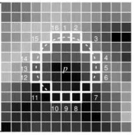
Bresenham’s Circle Drawing Algorithm is a circle drawing algorithm that selects the nearest pixel position to complete the arc.

• To make the algorithm fast, first compare the intensity of pixels 1, 5, 9 and 13 of the circle with $I_p$
  • As evident from the example on the right, at least three of these four pixels should satisfy the threshold criterion so that the interest point will exist.
• If at least three of the four-pixel values $I_1, I_5, I_9, I_{13}$ are not above or below $I_p + t$, then $p$ is not an interest point (corner)
  • In this case reject the pixel $p$ as a possible interest point.
• Else if at least three of the pixels are above or below $I_p + t$
  • then check for all 16 pixels and check if 12 contiguous pixels fall in the criterion.
• Repeat the procedure for all the pixels in the image.

Limitations of the FAST algorithm

• There are a few limitations to the algorithm
• First, for $n < 12$, the algorithm does not work very well in all cases, because when $n < 12$ the number of interest points detected are very high
• Second, the order in which the 16 pixels are queried determines the speed of the algorithm
• A machine learning approach can be added to the algorithm to deal with these issues

How ORB uses FAST as detector

• FAST or Features from Accelerated Segment Test is used as the key-point detector
• It works by selecting pixels in a radius around a key-point candidate and checks if there are n continuous pixels that are all brighter or darker than the candidate pixel
• This is made faster by only comparing a subset of these pixels before testing the whole range
• FAST does not compute orientation, to solve this the authors of ORB use the intensity weighted centroid of the key-point patch and the direction of this centroid with reference to the key-point is used as the orientation

How ORB uses BRIEF as descriptor

• BRIEF or Binary Robust Independent Elementary Features is used as the key-point descriptor.
• As BRIEF performs poorly with rotation, the computed orientation of the key-points are used to steer the orientation of the key-point patch before extracting the descriptor.
• Once this is done, a series of binary tests are computed comparing a pattern of pixels in the patch.
• The output of the binary tests are concatenated and used as the feature descriptor.

Example for ORB

import numpy as np
import cv2 as cv
from matplotlib import pyplot as plt

img = cv.imread('simple.jpg', cv.IMREAD_GRAYSCALE)

# Initiate ORB detector
orb = cv.ORB_create()

# find the keypoints with ORB
kp = orb.detect(img, None)

# compute the descriptors with ORB
kp, des = orb.compute(img, kp)

# draw only keypoints location, not size and orientation
img2 = cv.drawKeypoints(img, kp, None, color=(0,255,0), flags=0)
plt.imshow(img2), plt.show()

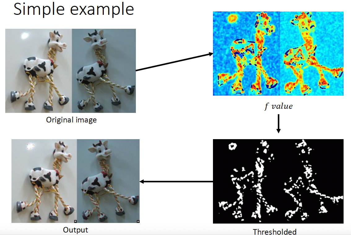
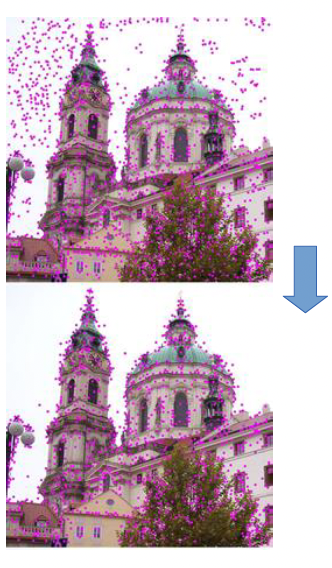
An application: Image matching

• We detect interest points to find a representation for an image
• We can then use this representation for different applications
• For instance
  • To match two image perspectives of the same scene
  • To track targets of interest, for instance in physical security
  • To match the left and right view taken by a stereo camera, to determine the depth of a given target or parts of a scene
  • To create a mosaic of a series of frames used to build a panoramic view, for instance with your smart device

Key Requirement - Invariance

Suppose we are comparing two images I₁ and I₂

• I₂ may be a transformed version of I₁
• What kinds of transformations are we likely to encounter in practice?

Want to find the same features regardless of the transformation

• This is called transformational invariance
• Most feature methods are designed to be invariant to
  • Translation, 2D rotation, scale
• They can usually also handle
  • Limited 3D rotations (SIFT works up to about 60 degrees)
  • Limited affine transformations (some are fully affine invariant)
  • Limited illumination/contrast changes

Achieving invariance ….

Need both of the following:

1. Make sure your detector is invariant
   • Harris is invariant to translation and rotation
   • Scale is trickier …. use SIFT
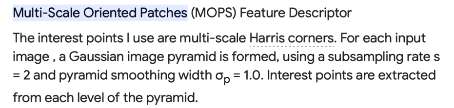
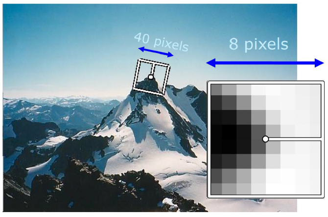
     • common approach is to detect features at many scales using a Gaussian pyramid (e.g., MOPS)
     • more sophisticated methods find “the best scale” to represent each feature (e.g., SIFT)

1. Design an invariant feature descriptor
   • A descriptor captures the information in a region around the detected feature point
   • The simplest descriptor: a square window of pixels
     • What’s this invariant to?
   • Let’s look at some better approaches…

Rotation invariance for feature descriptors

Find dominant orientation of the image patch

• This is given by $x_*$, the eigenvector of $H$ corresponding to $\lambda_+$ is the larger eigenvalue
• Can rotate / align the descriptor image patch according to this angle

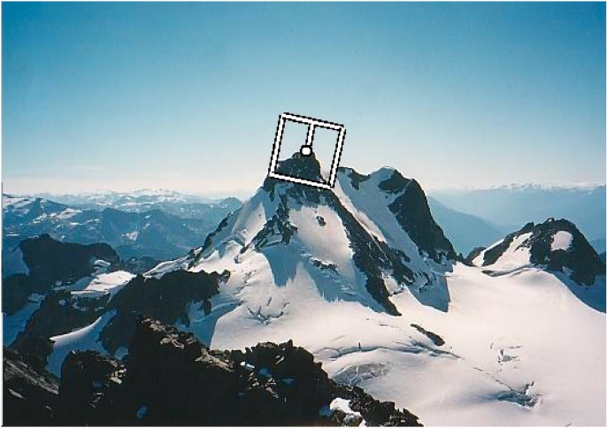
Multiscale Oriented Patches descriptor

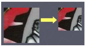
Take 40x40 square window around detected feature

• Scale to 1/5 size (using pre-filtering)
• Rotate to horizontal
• Sample 8x8 square window centered at feature
• Intensity normalize the window by subtracting the mean, dividing by the standard deviation in the window → then compare pixels

SIFT Feature Matching

• Given a feature in $I_1$, how to find the best match in $I_2$?
  • Define distance function that compares two descriptors
  • Test all the features in $I_2$, find the one with min distance

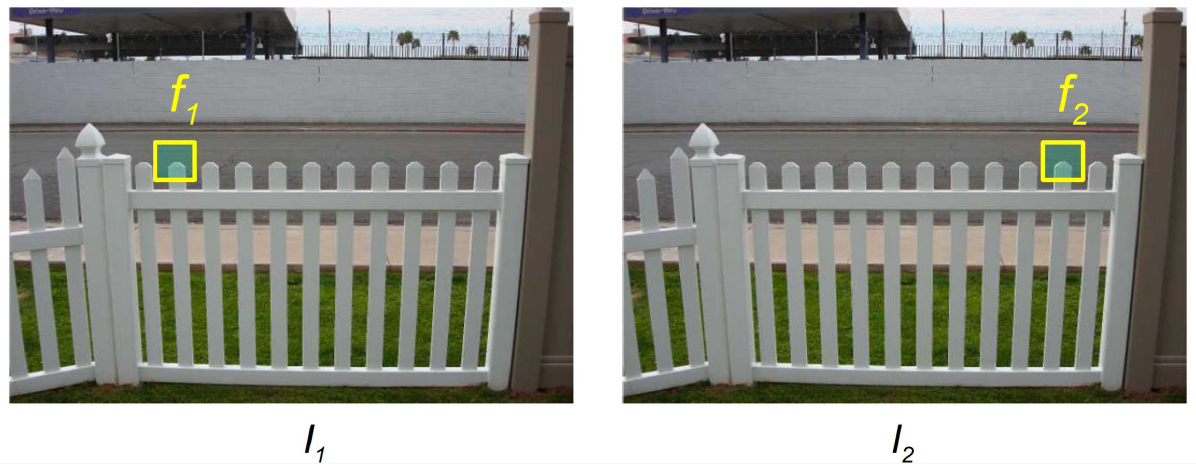
Feature Distance

How to define the difference between two features $f_1, f_2$?

• Better approach: ratio distance = $\text{SSD}(f_1, f_2) / \text{SSD}(f_1, f_2’)$
  • $f_2$ is best SSD match to $f_1$ in $I_2$
  • $f_2’$ is 2nd best SSD match to $f_1$ in $I_2$
  • gives small values for unambiguous matches

Sum of squared differences (SSD) is a measure of match based on pixel by pixel intensity differences between the two images.

SIFT Feature Distance

• Efficiency
  • can compare features as N-Dimensional vectors in R^N using k-D trees (nearest neighbour search)
    • Query f₁ to fᵢ response in linear time
  • several optimisations on this approach
• Original SIFT approach [Lowe 2004]
  • variation on k-D tree approach
  • probability of match correct = ratio of 1st nearest match to 2nd nearest match
    • Reject all matches with ratio > 0.8
  • Effect = eliminates ~90% of false matches, discards ~5% of correct matches, only very “unique” matches are kept

Summary

• We have learnt about old and new algorithms to detect interest points in an image
• We have covered Moravec, Harris, Shi and Tomasi’s corner detectors
• We have learnt of more recent interest point detectors, including SIFT, SURF and ORB
• We have started looking at how to match images using interest points

[[2025-01-20-CV-4]]