CV Lecture 4

CV Lecture 4

Image segmentation

• The process of segmenting an image into parts or fragments and assigning a label to each of those
• Three are the basic types of image segmentation
  • Instance segmentation
  • Semantic segmentation
  • Panoptic segmentation

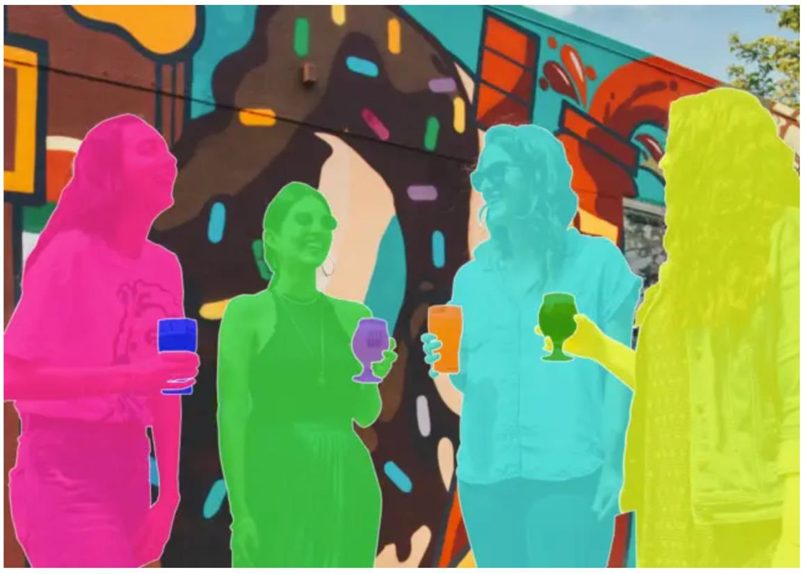
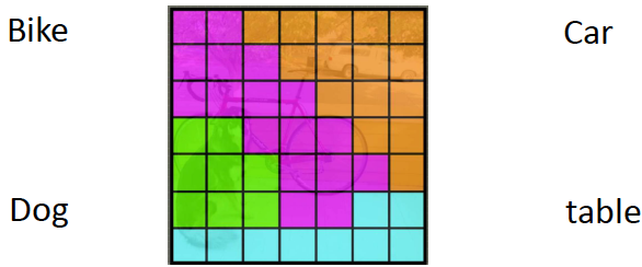
Instance segmentation

• Objects with their bounds are detected in the image
• However, each new object is labelled as a different instance, even within the same category

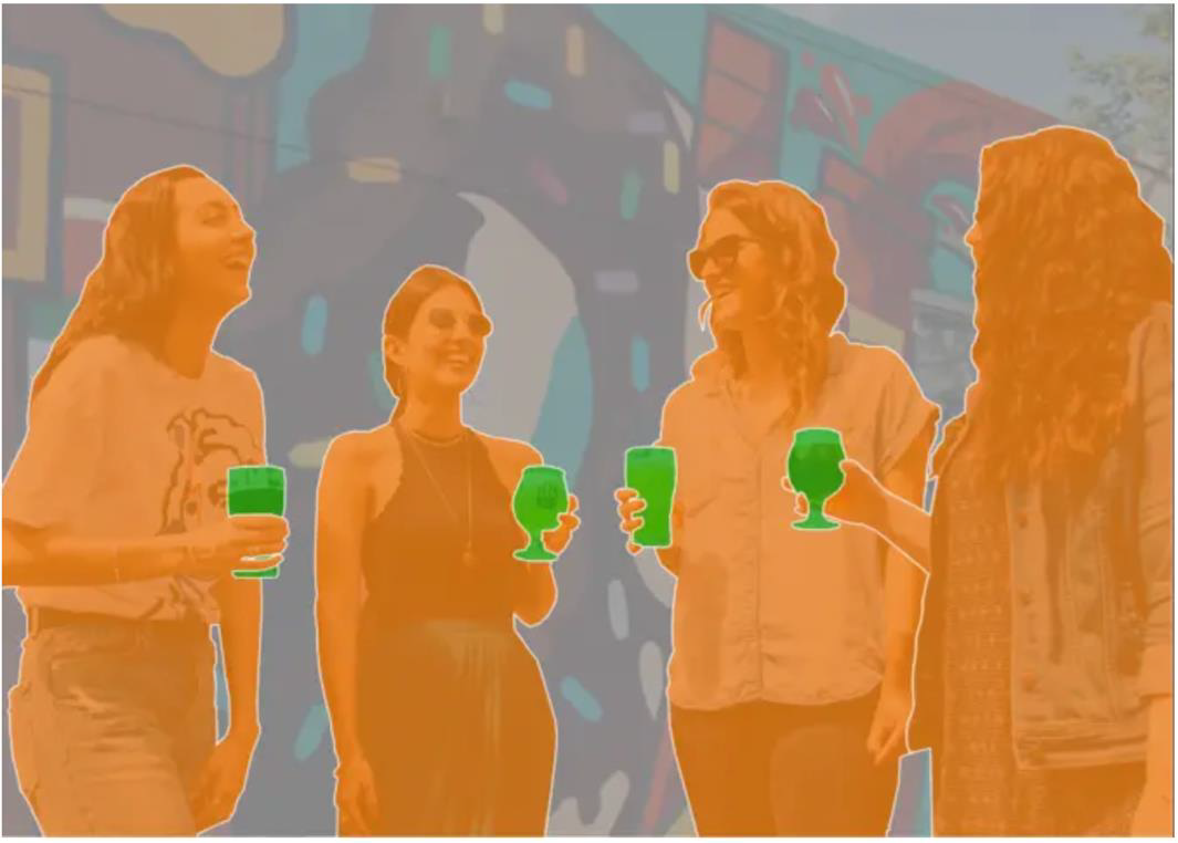
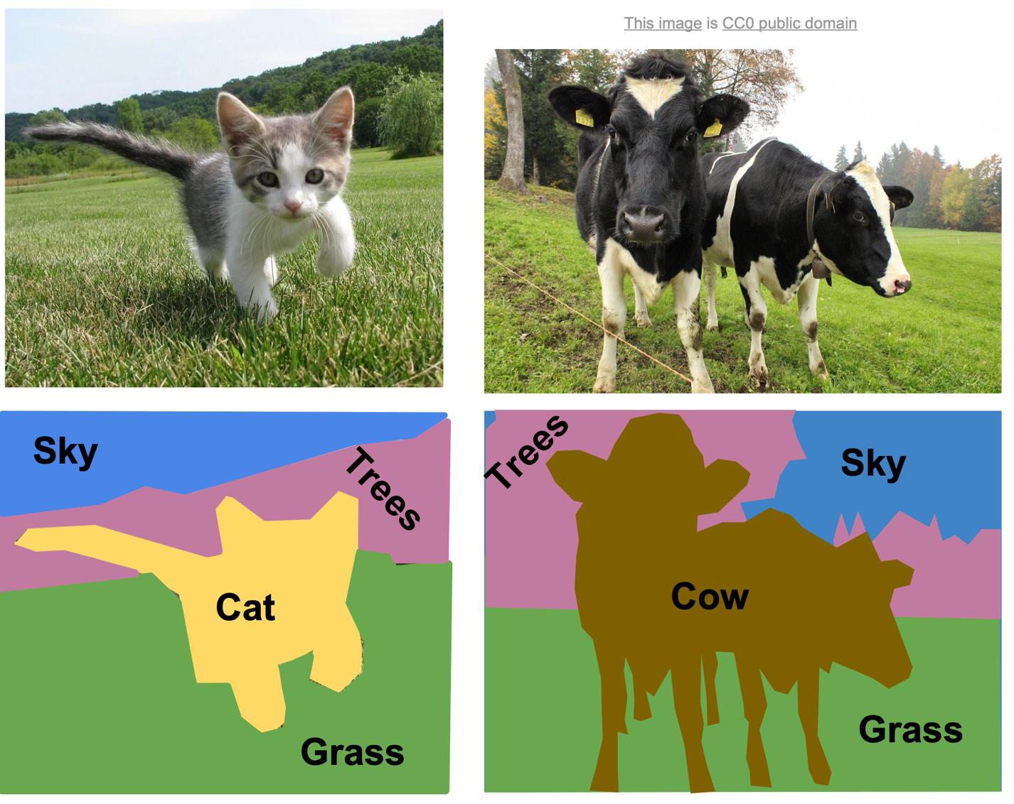
Semantic segmentation

• Segmentation masks represent fully labelled images
• It means that all pixels in the image should belong to some category, whether they belong to the same instance or not
• However, in this case, all pixels with the same category are represented as a single segment

Another example

• Label each pixel in the image with a category label
• Do not differentiate instances, only care about pixels

Panoptic segmentation

• It is a combination of both instance segmentation and semantic segmentation
• With panoptic segmentation, the entire image should be labelled
• Pixels from different instances should have different values even if they have the same category

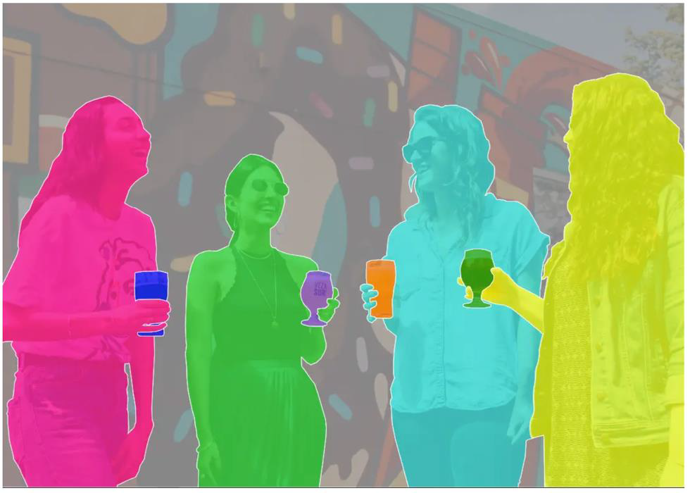
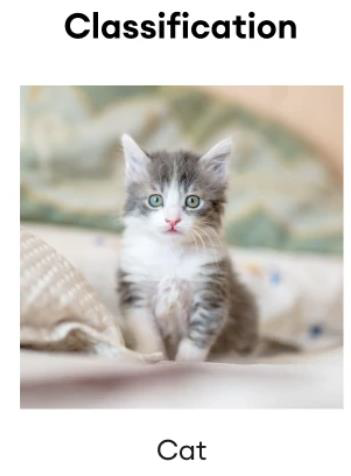
Image classification

A single class is assigned to an image, commonly to the main object that is portrayed in the image.

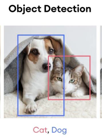
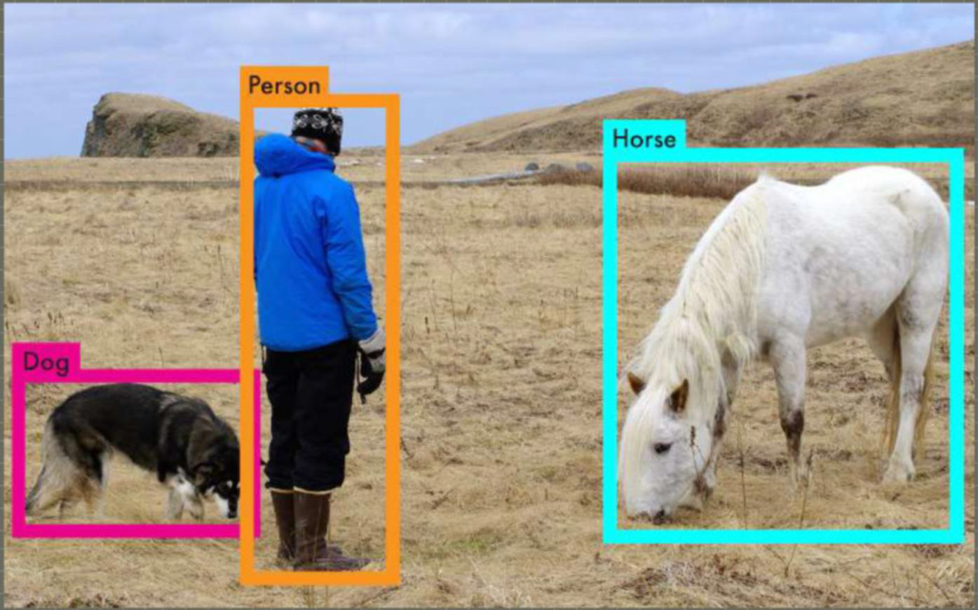
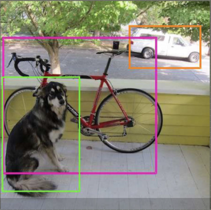
Object detection

• The objects within an image or a video are detected
• They are also marked with a bounding box, and then labelled

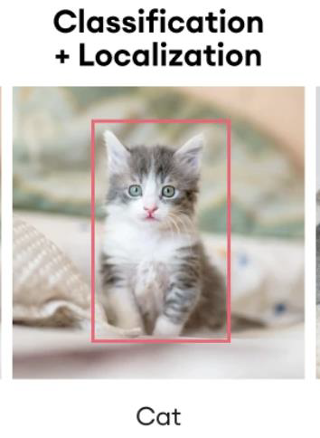
Localization

• Image object localization identifies the location of the main subject of an image
• However, image localization does not typically assign classes to the localized object as it considers the main subject instead of all of the present objects in a given frame
• We can combine localization with classification

Traditional Image Segmentation Methods

• Region-based segmentation
  • We have seen colour segmentation
• Edge detection segmentation
  • We have seen several methods, including Sobel, Canny
• Thresholding
  • We could use thresholds to define a colour
  • Check this link
• Clustering
  • We have seen the K-means

Hough Transform

• Check this nice presentation
  Hough Transform Presentation

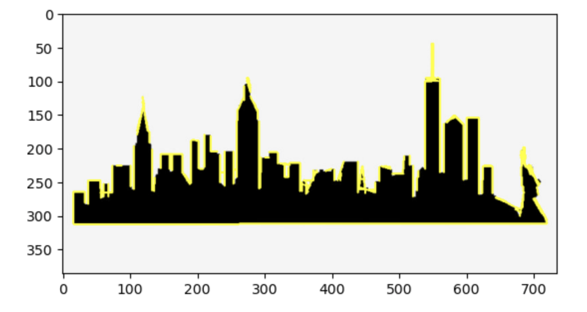
import cv2
import numpy as np
import matplotlib.pyplot as plt

# Read image
image = cv2.imread('SKYLINE1.jpeg')

# Convert image to grayscale
gray = cv2.cvtColor(image, cv2.COLOR_BGR2GRAY)

# Use canny edge detection
edges = cv2.Canny(gray, 50, 150, apertureSize=3)

# Apply HoughLinesP method to
# directly obtain line end points
lines_list = []
lines = cv2.HoughLinesP(
    edges,           # Input edge image
    1,               # Distance resolution in pixels
    np.pi/180,      # Angle resolution in radians
    threshold=10,    # Min number of votes for valid line
    minLineLength=5, # Min allowed length of line
    maxLineGap=10    # Max allowed gap between line for joining them
)

# Iterate over points
for points in lines:
    # Extracted points nested in the list
    x1, y1, x2, y2 = points[0]
    # Draw the lines joining the points
    cv2.line(image, (x1, y1), (x2, y2), (255, 255, 0), 2)
    
    # Maintain a simples lookup list for points
    lines_list.append([(x1, y1), (x2, y2)])

# Save the result image
cv2.imwrite('detectedLines.png', image)
plt.imshow(image)

Hough Transform example

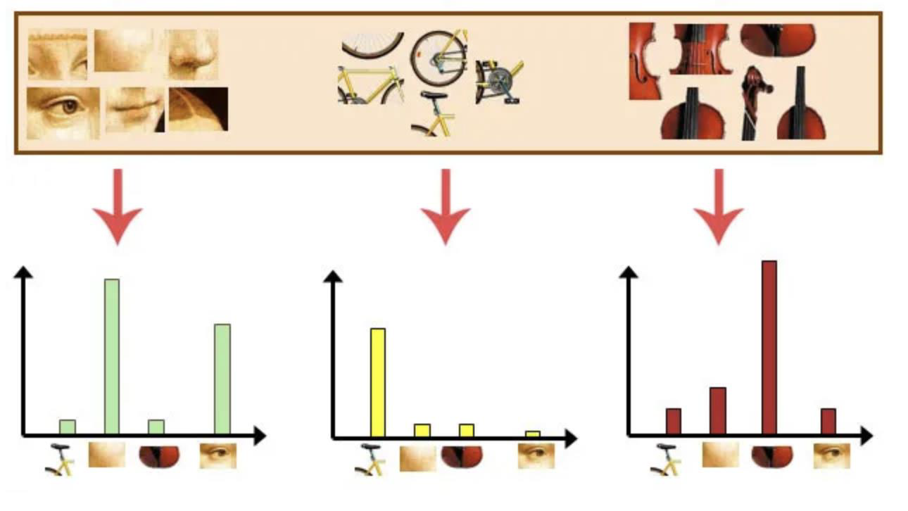
Bag of words

• Bag of words is an algorithm in natural language processing (NLP) that was designed to classify documents
• A bag is a sparse vector of occurrence counts of words
  • A histogram over a given vocabulary
• Bag of visual words makes use of features as words
  • A histogram over a given visual vocabulary

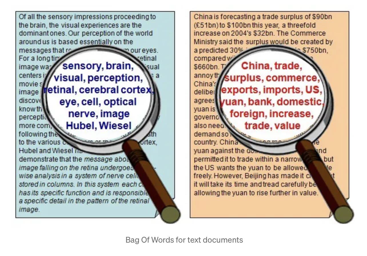
Bag of Words (NLP)

• In Bag Of Words, we scan through the entire document
• Keep a count of each word appearing in the document
• Then, we create a histogram of frequencies of words and
• Use this histogram to describe the text document

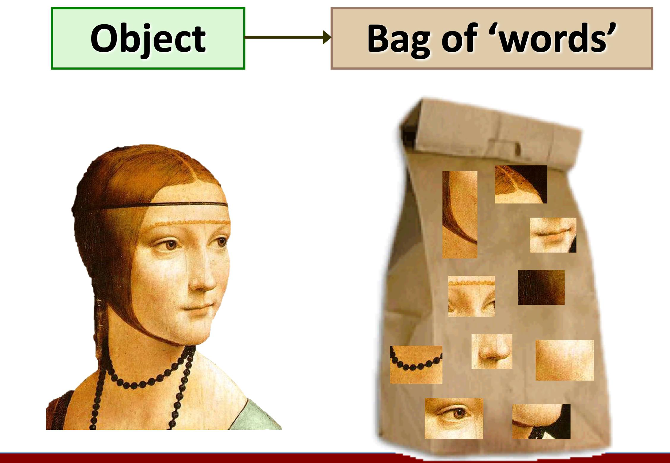
Bag of Visual Words (BoVW)

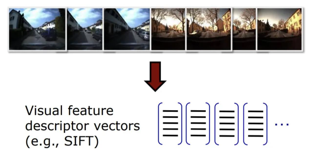
• In BoVW, we breakdown our image into a set of independent features
• Features consists of key points and descriptors
• Key points are the same thing as interest points
• They are spatial locations, or points in the image that define what is interesting or what stand out in the image
• They are invariant to image rotation, scale, translation, distortion etc.

Words: key points and descriptors

• Key points (interest points) are specific points in an image, say every 10th pixel in an image
• Descriptors are the values (description) of that key points
• We then create a dictionary or codebook based on these descriptors using clustering algorithms
• We reiterate through our images and check whether our image has words present in the dictionary
  • If so, we increase the count of that particular word
• Finally, we create the histogram for this image

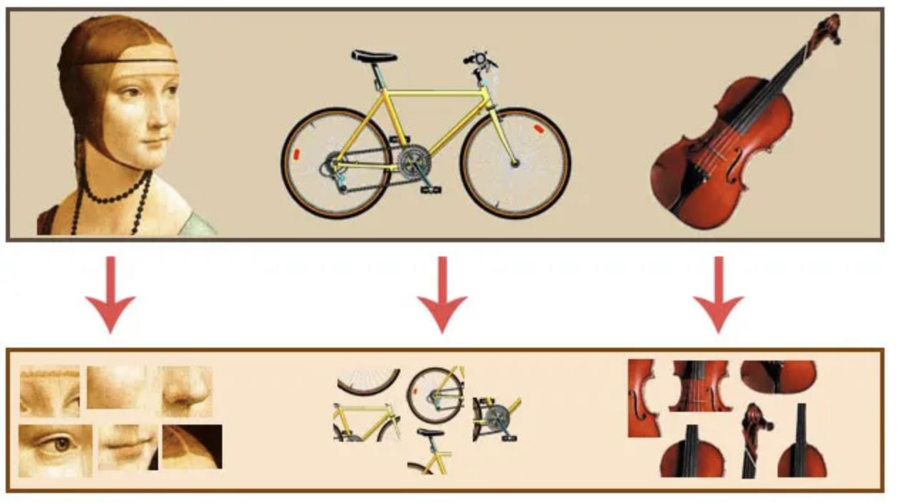
From images to visual words

• An image can be broken down in a number of features
• Features consist of interest points and descriptors

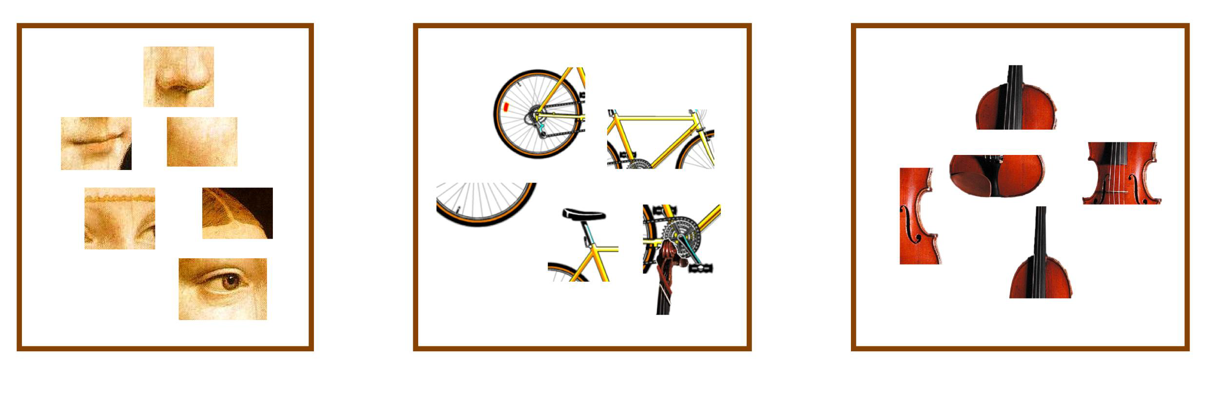
Bag of Visual Features: Feature Extraction

Storing feature frequencies

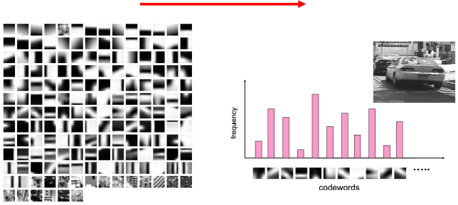
• Invariant interest points and their descriptors are used to construct vocabularies
• Each image is therefore represented as a frequency histogram of features

Building a visual dictionary

• We detect features, extract descriptors from each image in the dataset
• Detecting features and extracting descriptors in an image can be done by using feature extractor algorithms (for example, SIFT, SURF, ORB …)

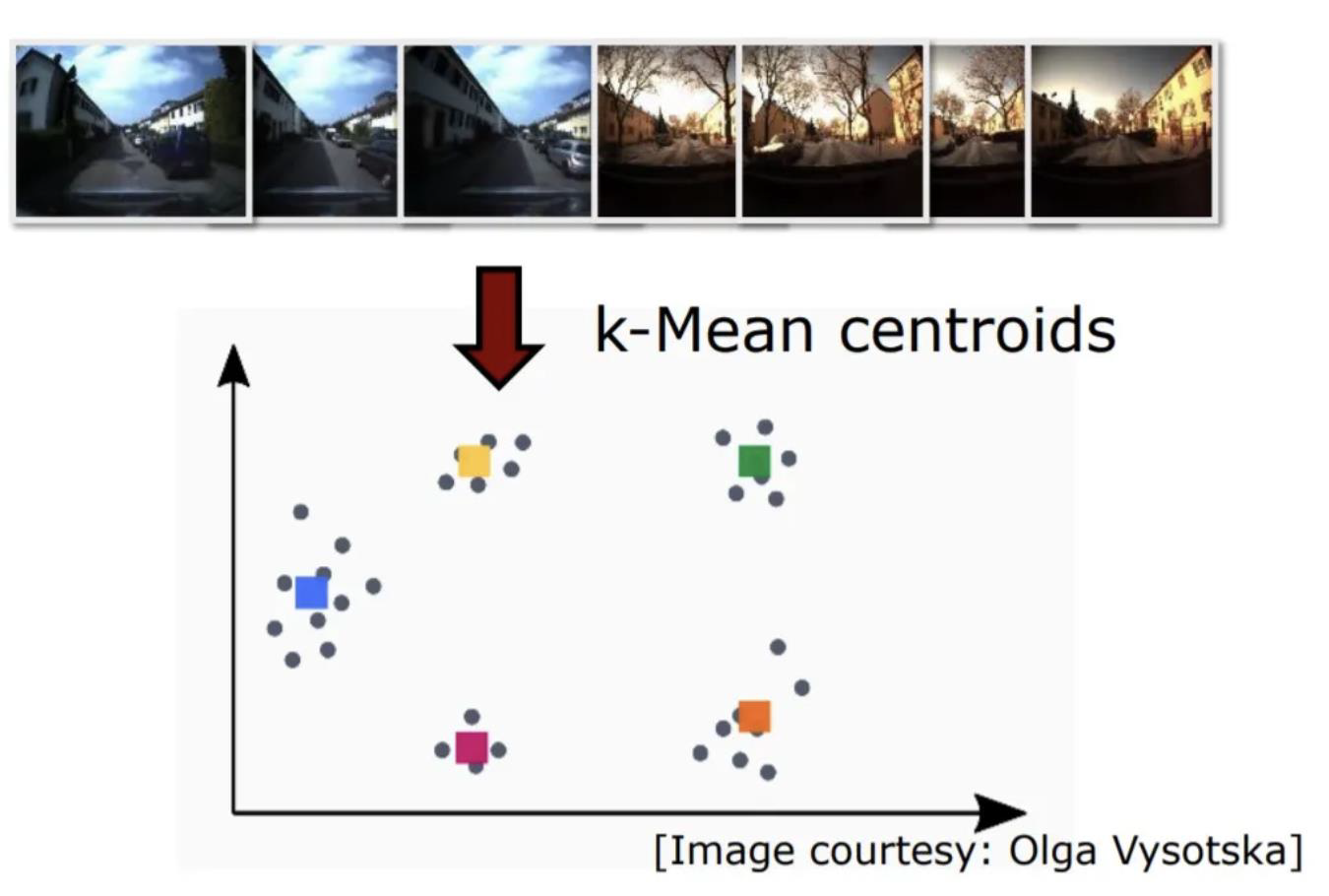
From descriptors to clusters

• We make clusters from the descriptors
  • we can use K-Means, or another clustering algorithm)
• The centre of each cluster will be used as the visual dictionary’s vocabularies

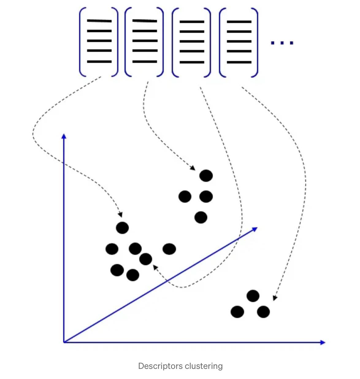
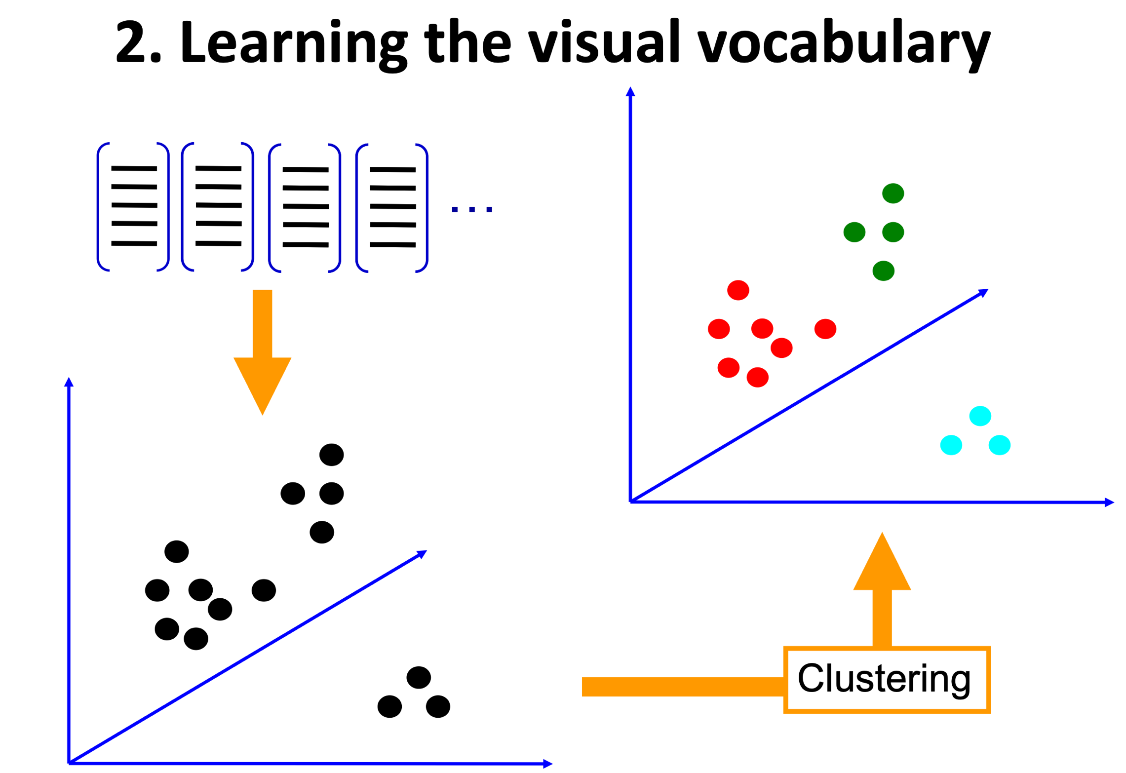
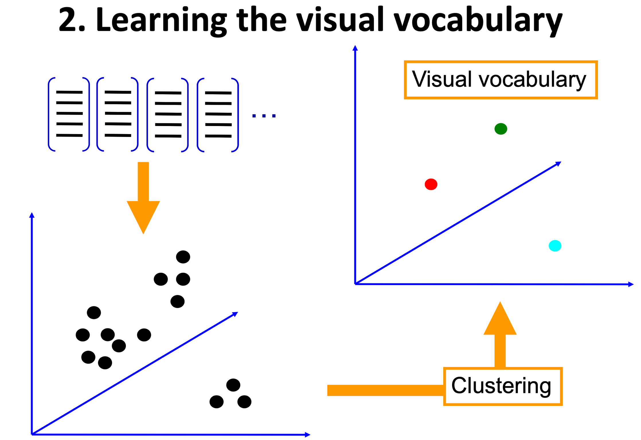
• K-Means groups the data points into K groups and will return the centre of each group (see image below)
• Each cluster centre (centroid) acts as a visual word
• All these K centroids form our codebook

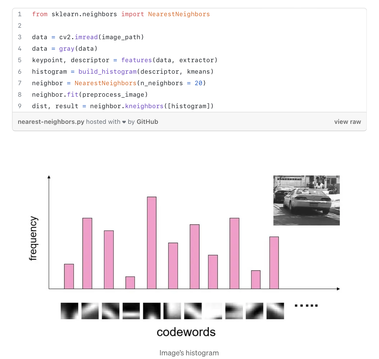
From vocabulary to image representation

Problems with BoVW

• If a feature appears in too many images, or all of them, it is no longer significative
• A solution to this problem is to scale down the importance of these features, essentially reweighting every bin of a histogram that is related to “uninformative” words
• Vocabulary size is also a problem
  • Too small: the visual words are not representative of all parts of an image
  • Too large: too much detail is present, resulting in overfitting

Modern Computer Vision methods

• Since the recent success of machine learning, there has been a noteworthy shift
• I have already mentioned this in a previous lecture
• At present, most algorithms/methods use deep neural networks
• Neural networks are very old computational algorithms
• They disappeared almost entirely until deep networks were proposed and proved superior performance with respect to traditional methods

From real/animal to artificial neurons

• Artificial neurons are rooted in some old research by Santiago Ramon y Cajal’s theory of dynamic polarization of nerve cells, in 1888
• Charles Scott Sherrington coined the term synapse in 1897, to name what Cajal described the interneural contact

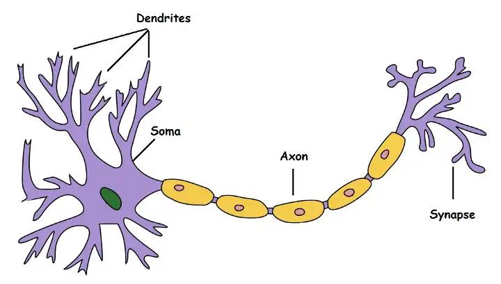
First computational model of the neuron

In 1943, Warren S. McCulloch and Walter Pitts contended that neurons with a binary threshold activation function were analogous to first order logic sentences.

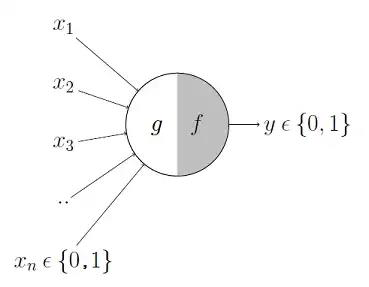
How does their model work?

• The process is divided in two parts
  • In the first part, g takes an input (dendrite)
  • Then, g performs an aggregation
  • Based on the result, f makes a decision

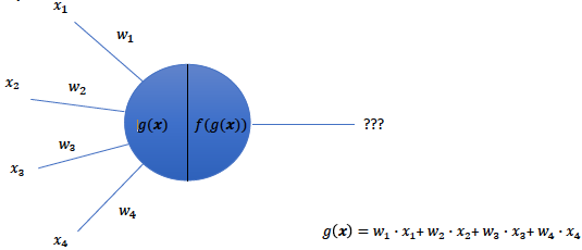
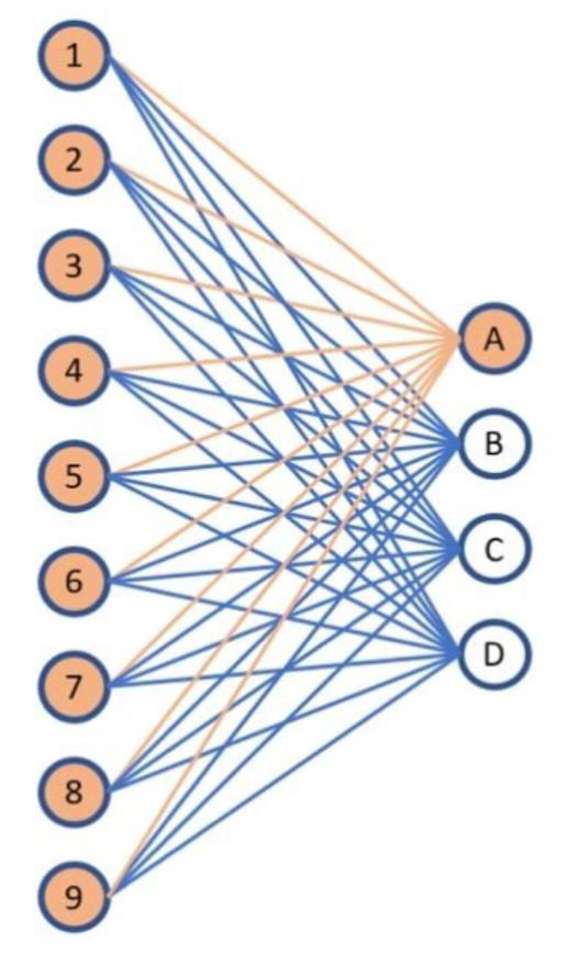
What if each input had a different importance?

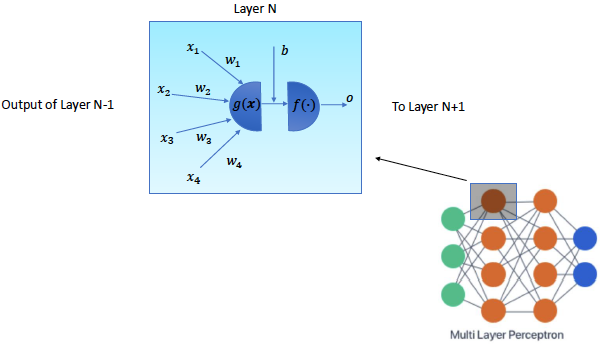
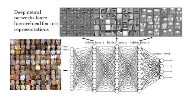
Artificial Neural Network

• By adding a hidden layer, we have the implementation of an artificial neural network
• Artificial Neural Networks, abbreviated ANN, or simply NN, are defined by a number of parameters that define its topology
  • Number of layers
  • Number of neurons per layer
  • Connections between layers
  • Activation functions

Why do we use more layers?

Deep networks work very well

• There is no sense in using old methods any more
• Deep networks are superior
• Check this example

How do neural networks work?

• Neural networks in generals are non-linear approximators
  • An image in input is processed and layer by layer a more specific representation is built
  • Information passed between neurons is combined with weights
  • Weights are learnt
• Three are the basic phases
  • Training: during this phase, a large dataset is used to learn the weights
  • Validation: during this phase, hyperparameters are tuned to find the better model
  • Testing: images not from the training set are used to test the performance of the neural network

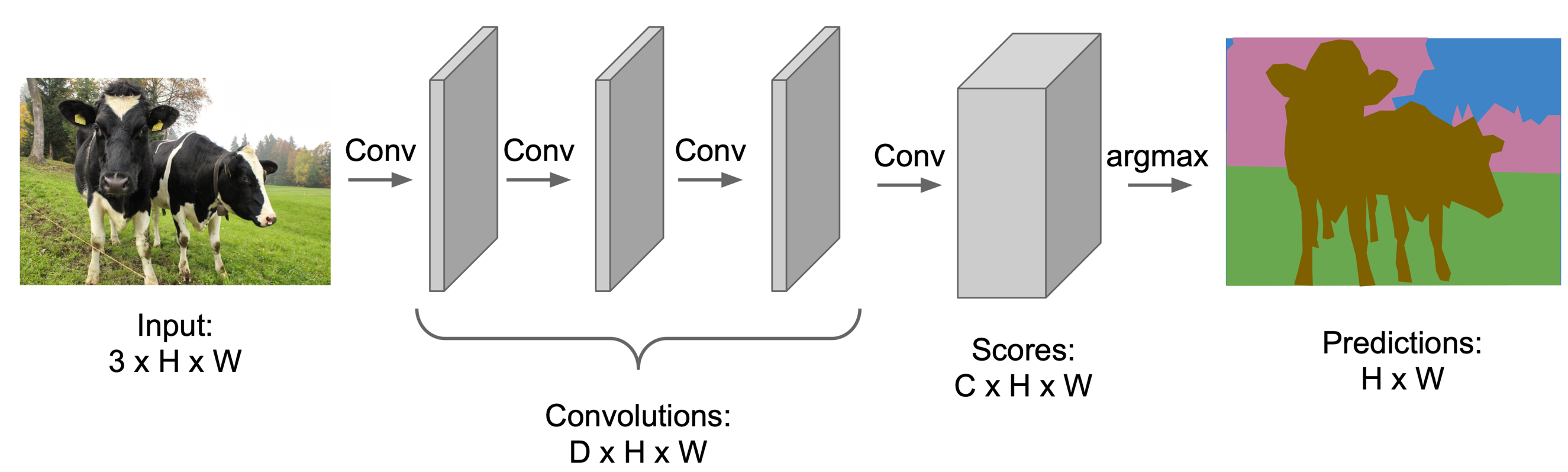
Semantic segmentation with a CNN

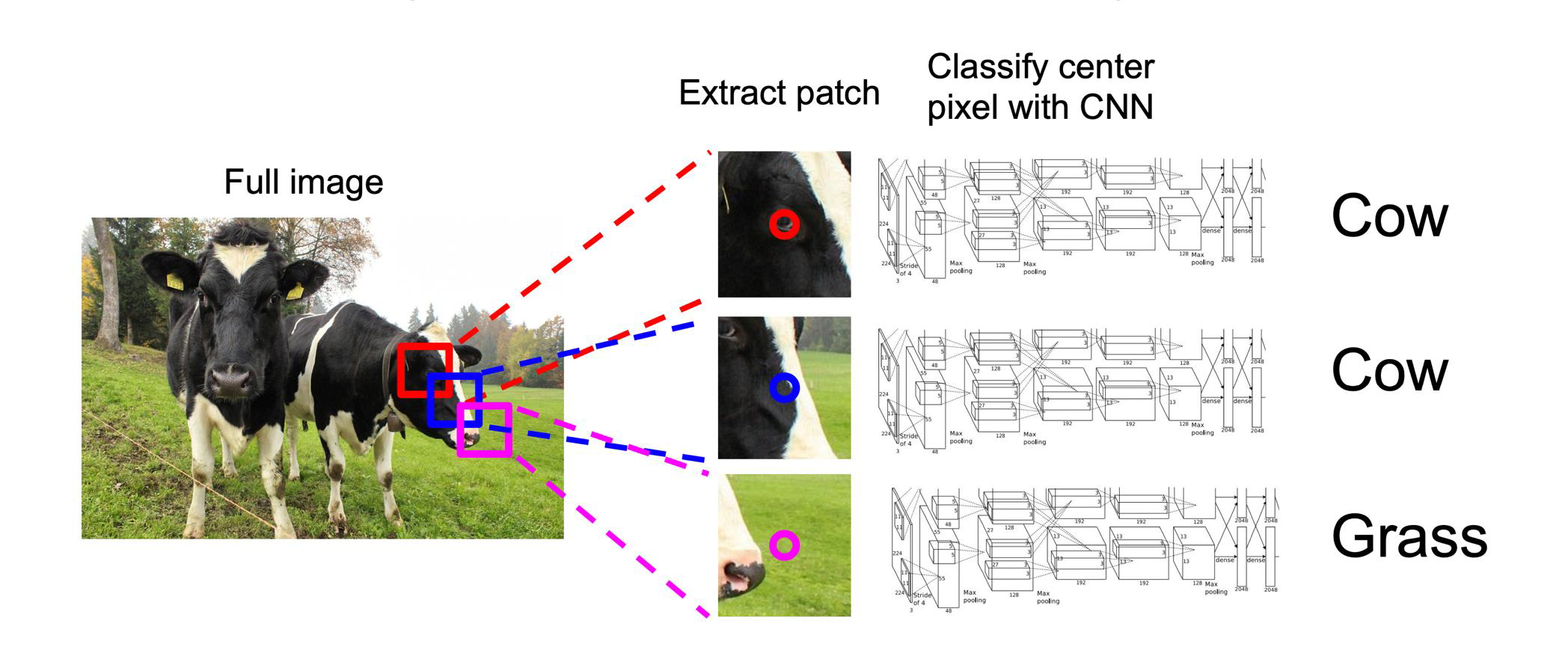
Too slow: very inefficient!

Convolutions at image resolution are very expensive.

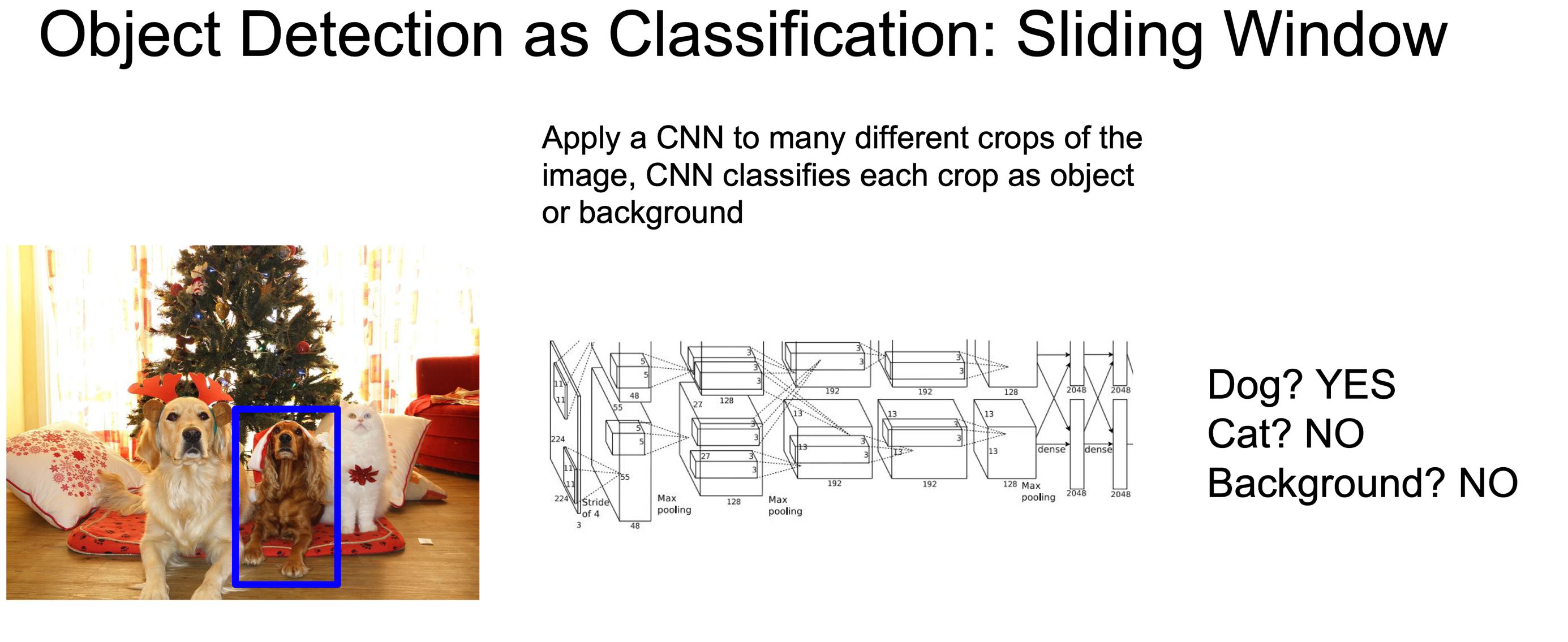
These methods use what is called Exhaustive Search which uses sliding windows of different scales on an image to propose region proposals.

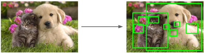
Region Proposals

• Find “blobby” image regions that are likely to contain objects
• Relatively fast to run; e.g. Selective Search gives 1000 region proposals in a few seconds on CPU

AlexNet

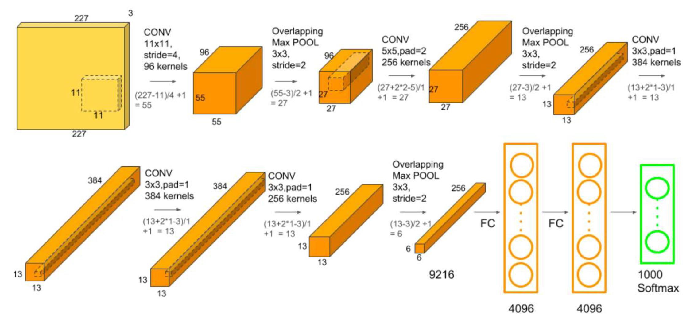
AlexNet on ImageNet

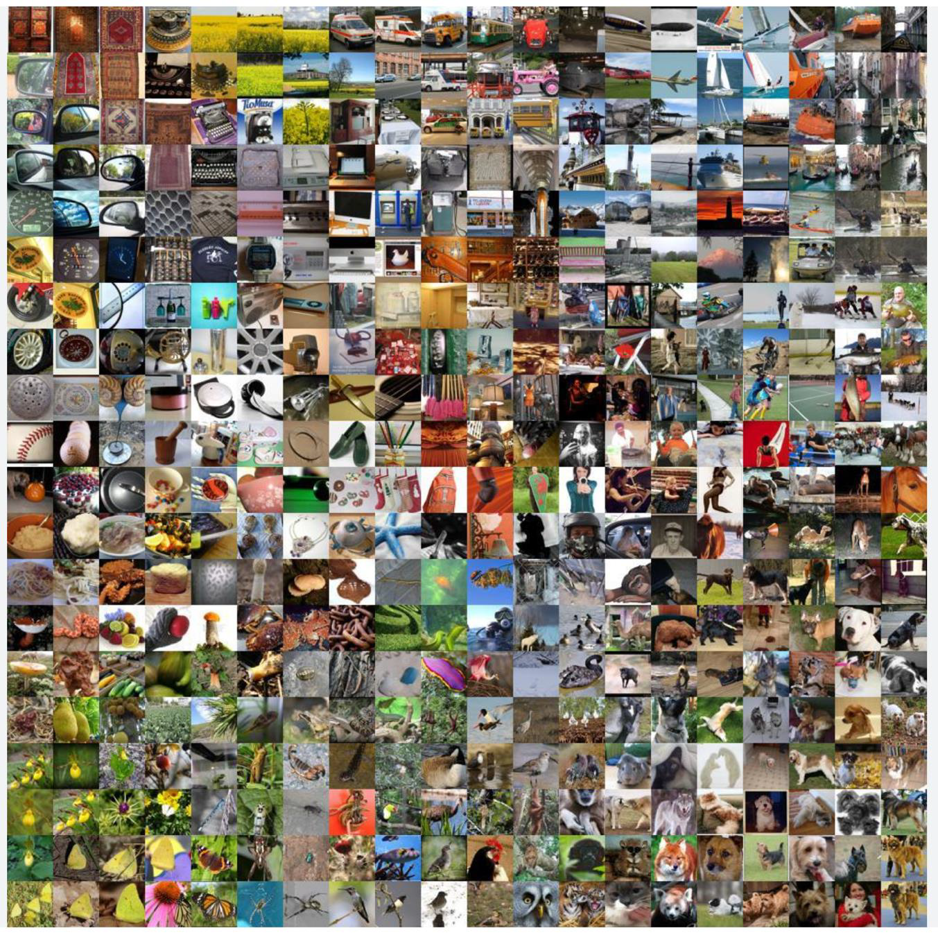
ImageNet dataset contains 14,197,122 annotated images according to the WordNet hierarchy. Since 2010, the dataset is used in the ImageNet Large Scale Visual Recognition Challenge (ILSVRC), a benchmark in image classification and object detection.

AlexNet

• Fully connected layer

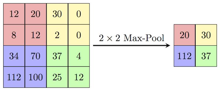
• Max Pooling
  • calculates the maximum value for patches of a feature map, and uses it to create a downsampled (pooled) feature map

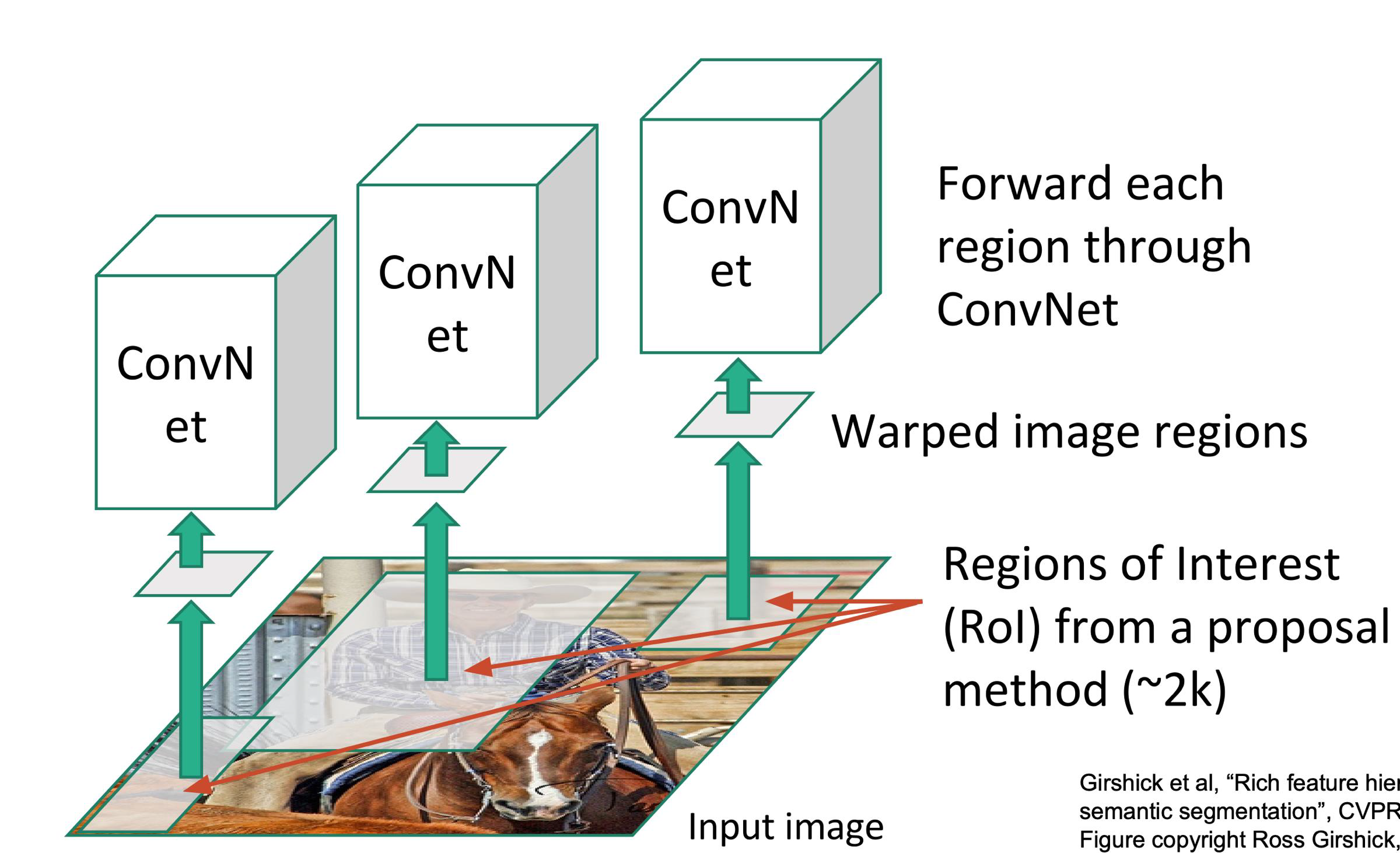
The Region based CNN (R-CNN) algorithm

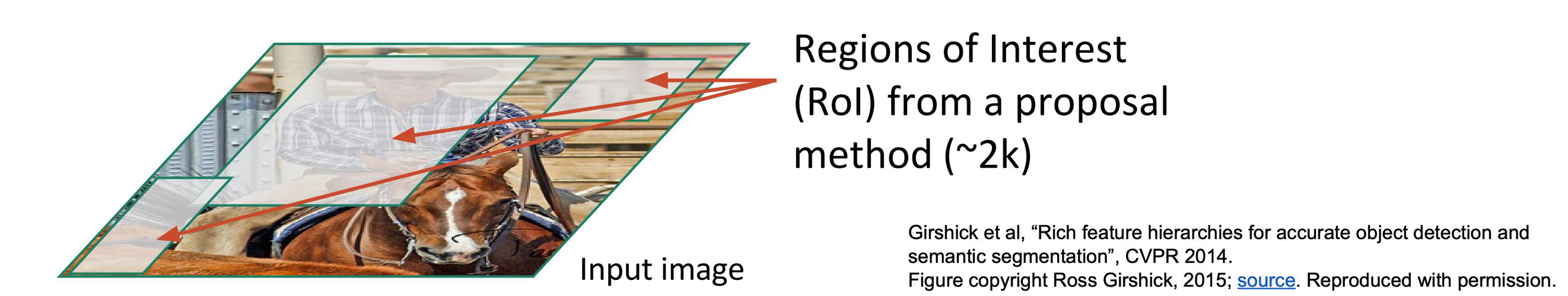
• This time CNN are run on a set of regions of interest, usually called proposals
• Proposals might be in a number as large as 2K
• They can be detected using various methods
• They are the basis of this algorithm, as they speed up the processing

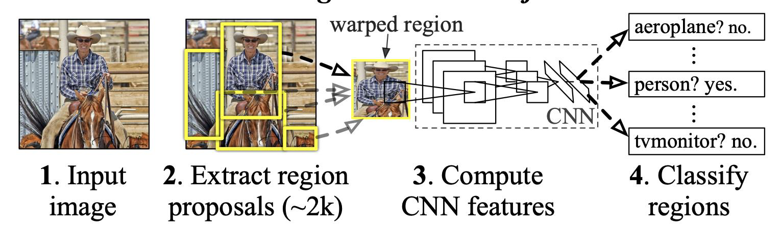
R-CNN steps

• An image is input.
• Around 2000 regions of interest (proposals) are extracted bottom-up.
• For each proposal, fixed length feature vectors are extracted using a large convolutional neural network (CNN).

Classification with SVMs

R-CNN problems

• Each image needs to classify 2000 region proposals
  • So, it takes a lot of time to train the network
• It requires 49 seconds to detect the objects in an image on GPU
• To store the feature map of the region proposal, a lot of Disk space is also required

Fast R-CNN

• R-CNN is passed each region proposal one by one in the CNN architecture
  • it is computationally expensive to train and even test
• Fast R-CNN takes the whole image and region proposals as input in one forward propagation

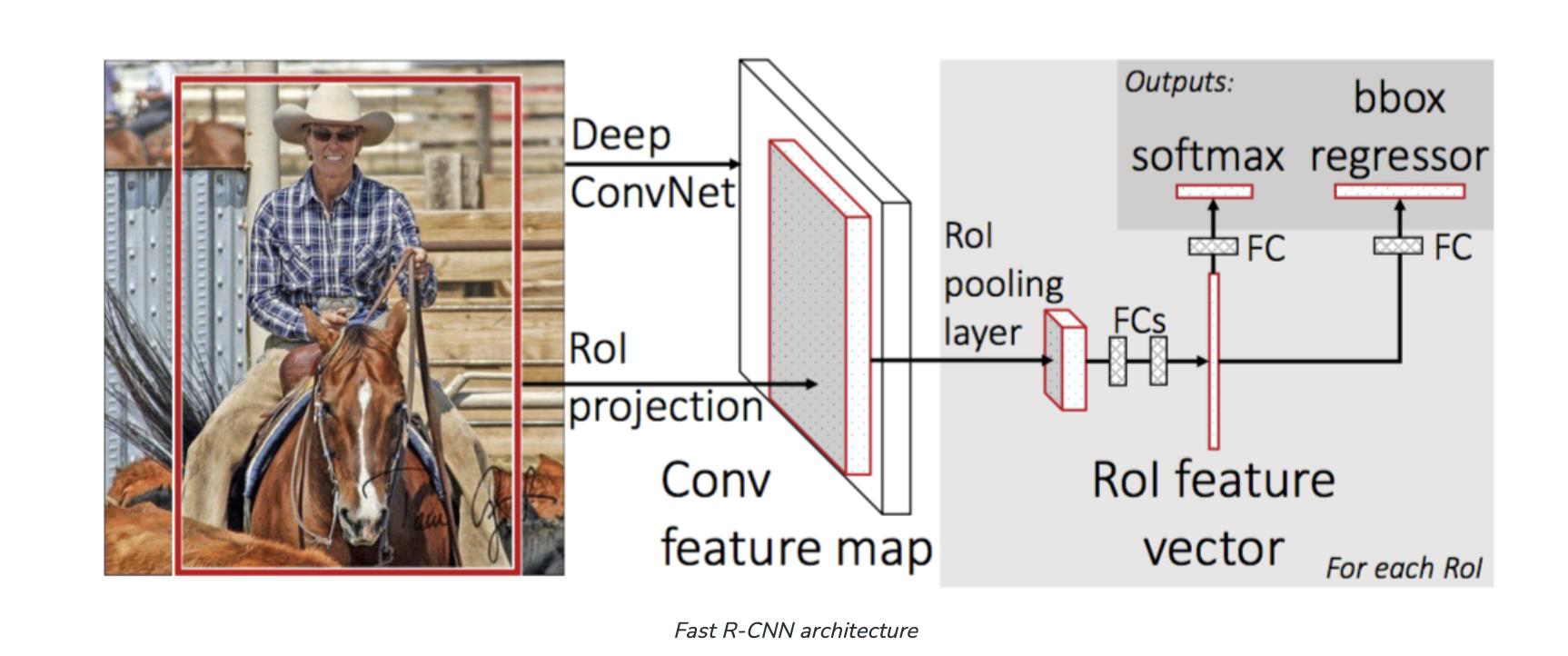
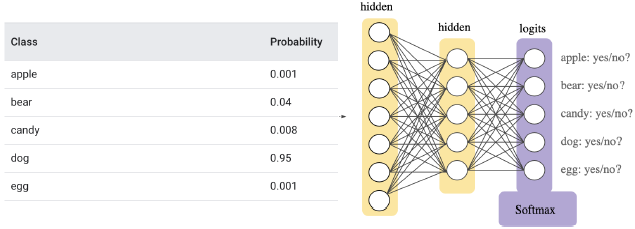
Fast R-CNN uses the softmax layer

• the softmax layer instead of SVM in its classification of region proposal which proved to be faster and generate better accuracy than SVM
• Softmax assigns decimal probabilities to each class in a multi-class problem
• Those decimal probabilities must add up to 1.0
• This additional constraint helps training converge more quickly than it otherwise would.

Softmax layer

• Softmax is implemented in a neural network layer just before the output layer
• The Softmax layer must have the same number of nodes as the output layer

Traditional and Modern methods

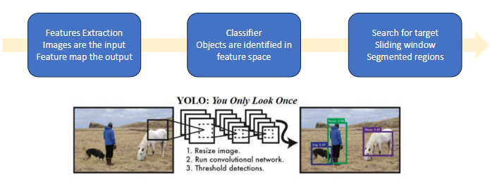
You Only Look Once (YOLO)

• YOLO runs in real time, it is one of the faster algorithms
• It can be used in several applications
  • Autonomous driving
  • Assistive devices
  • Robotic rovers

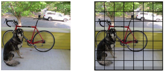
How does YOLO work?

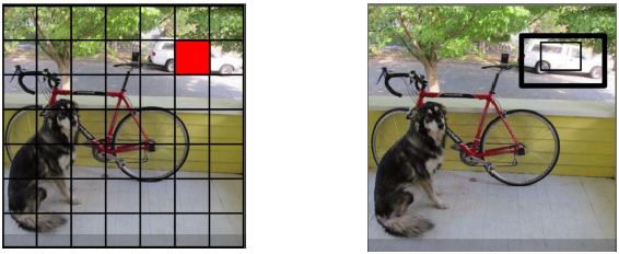
• An image is split into cells, say SxS
• If the centre of an object falls in a given cell, that cell is responsible for recognizing the object

• Each cell predicts B bounding boxes and C class conditional probabilities $P(class_i

  object)$

• Each bounding box consists of x, y, w, h and confidence
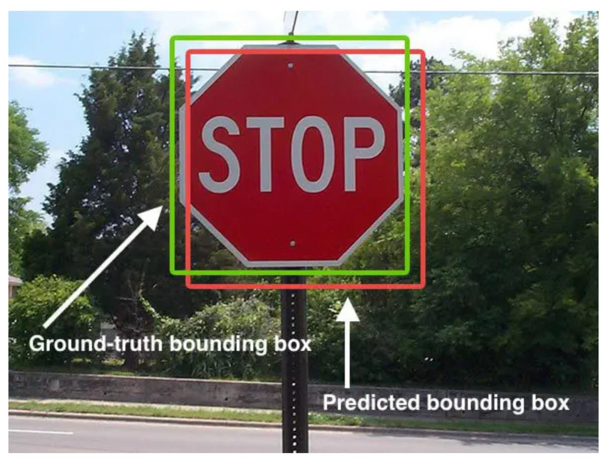
• Confidence = $P(object) \cdot IOU$
• IOU is the intersection over union between prediction and ground truth

Intersection over Union

• More details at
  pyimagesearch.com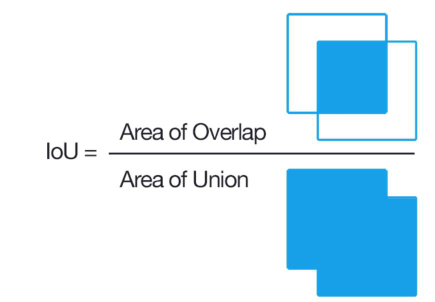

• The conditional probabilities and individual box confidence predictions are multiplied
  • This yields class specific confidence scores for each box
• A score encodes
  • Probability of a specific class to appear in the box
  • How well the predicted box fits the object

\[P(class_i|object) \cdot P(object) \cdot IOU\left(\frac{truth}{pred}\right) = P(class_i) \cdot IOU\left(\frac{truth}{pred}\right)\]

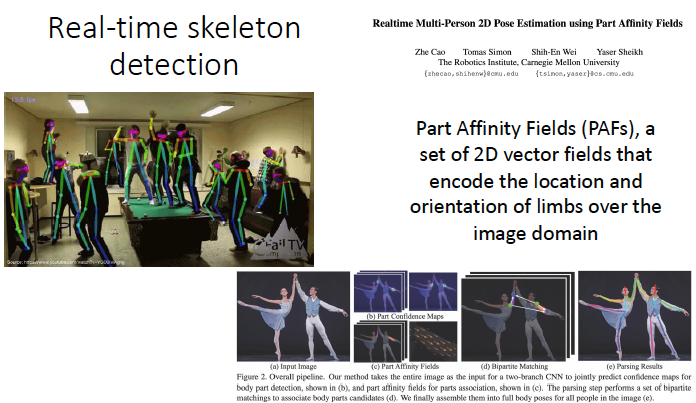
Skeleton detection

• Skeleton detection is a technique that recognizes and determines the essential points in the human body, including the top of the head, neck, shoulders, elbows, wrists, hips, knees, and ankles.
• Full-body and half-body static image recognition and real-time video stream recognition are already supported, and skeleton recognition affects system performance and algorithm complexity and is required for general shape representation.

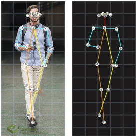
Detecting the skeleton of a person

• In order to detect a person, we can use many methods
• The deep networks we have seen today can do the trick
• We might want to have more information about a person
  • For instance, being able to extract their limbs (arms and legs)
• This because we might be interested in classifying the position and orientation of a person and classify also actions in a video

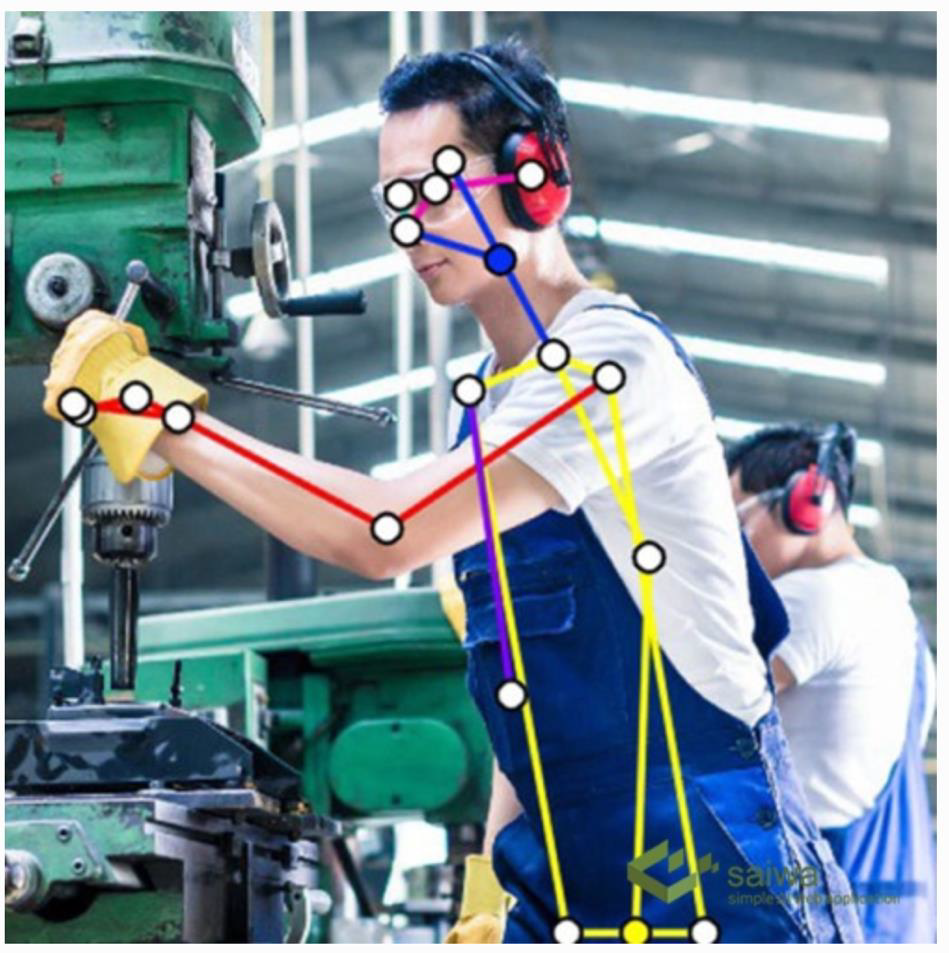
Skeleton detection algorithms

• OpenPose
  • A popular open-source library for detecting key points in the human body using a multi-stage CNN approach.
  • It can detect up to 135 critical points on the human body and has been widely used for gesture and action recognition applications.
• Mask R-CNN
  • A widely used object detection and segmentation algorithm that can also be used for skeleton detection.
  • It first uses a two-stage CNN approach to detect human bodies and then identifies the key points.

The U-net

• U-Net gets its name from its architecture
• The “U” shaped model comprises convolutional layers and two networks
  • First is the encoder, which is followed by the decoder
• With the U-Net, we can solve the above two questions of segmentation:
  • “what is the object” and “where is it”

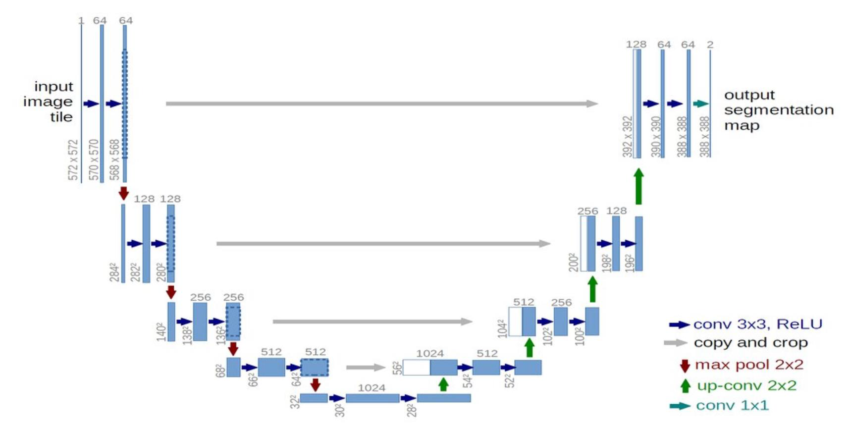
Encoder

• The encoder network is also called the contracting network
• This network learns a feature map of the input image and tries to solve our first question- “what” is in the image?
• It is similar to any classification task we perform with convolutional neural networks except for the fact that in a U-Net,
• It has no fully connected layers in the end, as the output we require now is not the class label but a mask of the same size as our input image

Decoder

• The decoder network is also called the expansive network
• The idea is to upsample the feature maps to the size of the input image
• This network takes the feature map from the bottleneck layer and generates a segmentation mask with the help of skip connections
• The decoder network tries to solve our second question—“where” is the object in the image?

U-net applications

• Biomedical Image segmentation
  • Brain image segmentation
  • Liver image segmentation
  • Protein binding site prediction
• Physical sciences
  • analysis of micrographs of materials
• Medical image reconstruction

Summary

• We learnt about object detection and classification
• We have studied the bag of visual words
• We have scanned over some of the most successful deep neural networks used for object detection, segmentation and classification