CV Lecture 5

CV Lecture 5

Tracking

• So far, we have studied methods to identify points of interest
  • … and their descriptors
• We have revisited traditional and modern methods
• We have studied methods where both scene and camera are stationary
• What if either of them moves or both move?
• In this lecture, we will study methods to track targets with a fixed camera, but where the scene is dynamic
  • Targets might move, whatever moves is called foreground, the rest is background

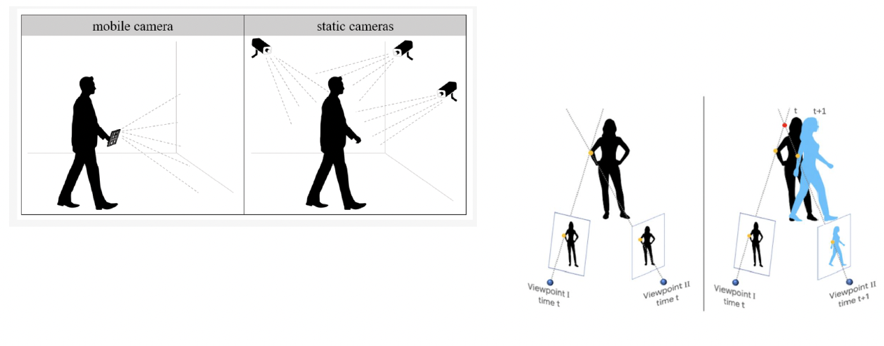
Static and moving cameras

Videos

• To study the dynamics of a scene we need to use a video camera
• A video, long or short, is a sequence of image frames 一系列图像帧
• Each frame can be analysed in isolation, or analysed in small batches to estimate the dynamics of the moving targets
• Applications abound:
  • Tracking individuals, groups of people or crowds in physical security
  • Tracking biological entities in a Petri dish
  • Tracking movement of animals in a protected area
  • Tracking athletes in games, such as football, rugby, tennis, skiing

Tracking individual targets

• In order to track a target, we need
  • To identify what needs to be tracked, this implies segmenting a scene in its main components and then selecting those of interest
    • 分割后选择感兴趣部分
  • Identification could be helped by seeding the tracking process, for instance a security guard might have identified a suspect, and an interactive user interface might allow the guard to click on the image region where the suspect is currently moving
• A target must be followed, this means to have an idea where it might go
  • This is called prediction
  • To be able and make predictions, we must be able to identify the target across frames and this might prove hard, especially if the target is in a very cluttered and crowded area 帧间识别目标

Tracking multiple targets

• What if we wanted to track more objects or people or combinations thereof?
• We would need
  • to have a method to identify each one of them
    • 识别每一个
  • To be able to make predictions for each one of their trajectories
    • 每一条轨迹作出预测
  • What if their trajectories are not simple and they intersect?
  • What if the targets are very similar?
• In a dynamic scene, even if captured by a stationary camera, targets enter and exit, not necessarily from the same area of the scene, some targets might exit and then re-enter …
  • 退出&进入

Additional problems

• A recorded scene might be indoors or outdoors
• If indoors, artificial lights, potentially mixed with external lighting might be flickering at a given frequency
• If outdoors, the scene is subject to natural elements: it could be a windy scene with overcast periods followed by sunny periods, illumination might be poor because the scene is recorded at the end of the day, it might be raining, snowing, hailing …etc.
• All those external elements would affect the scene and changes ought to be taken into consideration
  • 外部环境不一致

Moving targets in a stationary scene

• In the first instance, we need to identify the target, or targets to be tracked
• Let us say there is only one target, for instance a person moving in a stationary scene静态背景
• We have a video clip of this person moving
• We must identify what is moving

Background Modelling 背景建模

• One of the oldest methods in computer vision estimates the model what does not change
  • We called it background
• The method is called background modelling
• Once the background is modelled, then moving targets can be detected
  • These are commonly called foreground
• In practice, we are detecting changes
• Image frames have one or three channels, so change must be detected in all the channels
  • RGB

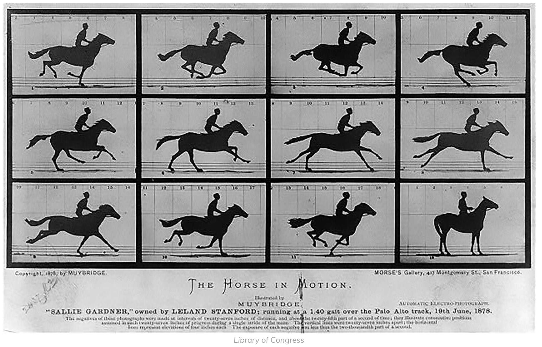
Frame rate and Object type problem

帧率和对象类型问题

• If the target is faster than the camera framerate, then the difference between two frames is useless as it contains a bit of both target position and orientation.
  • 快于帧率，则两帧之间的差异是无用的，因为它包含了目标位置和方向的一点
• For deformable objects, the matter gets even more complicated.
  • 对于可变形物体，情况变得更加复杂

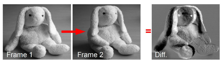
Detecting and Modelling Change

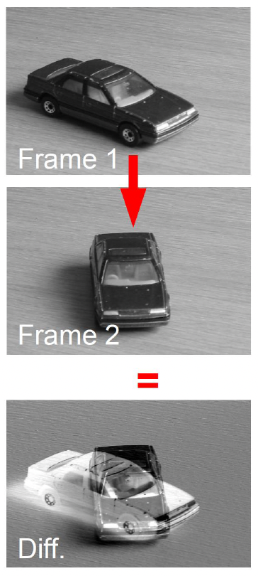
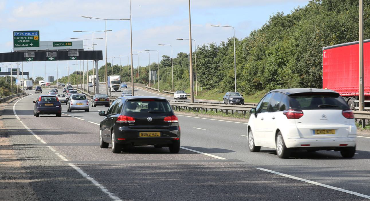
• The simplest methods to detect change is to take the difference between two images.
• If we do this, we will not see the full moving target, but only the portion of background the target has made visible while moving and the portion of background the target has now taken.
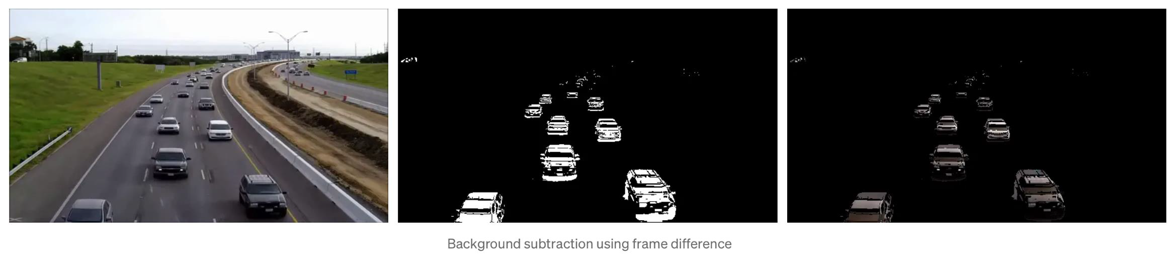
• Normally, we use a threshold. 设置阈值 Image(i) - Image(i-1) > threshold
• OpenCV can be employed to calculate the change.
  • See the next slide for the code and an example of car movement detection.

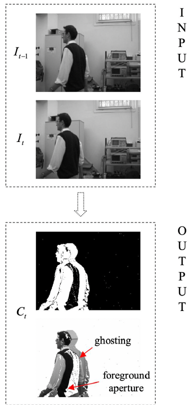
Ghosting Effect

• The output is a complex figure that mixes both the foreground and background.
• The halo effect surrounding the target is called ghosting.
  • 周围光晕

import numpy as np
import cv2 as cv

cap = cv.VideoCapture(0)
if not cap.isOpened():
    print("Cannot open camera")
    exit()
while True:
    # Capture frame-by-frame
    ret, frame = cap.read()
    # if frame is read correctly ret is True
    if not ret:
        print("Can't receive frame (stream end?). Exiting ...")
        break
    # Our operations on the frame come here
    gray = cv.cvtColor(frame, cv.COLOR_BGR2GRAY)
    # Display the resulting frame
    cv.imshow('frame', gray)
    if cv.waitKey(1) == ord('q'):
        break

# When everything done, release the capture
cap.release()
cv.destroyAllWindows()

cap = cv.VideoCapture(video)
ret, prev = cap.read()
prev = cv2.cvtColor(prev, cv2.COLOR_BGR2GRAY)
while(1):
    ret, frame = cap.read()
    gray = cv2.cvtColor(frame, cv2.COLOR_BGR2GRAY)
    frame_diff = cv2.absdiff(gray, prev)
    ret, thres = cv2.threshold(frame_diff, 35, 255, cv2.THRESH_BINARY)

    prev = gray.copy()
    cv2.imshow('original', frame)
    cv2.imshow('foregroundMask', thres)

Background subtraction using frame difference

Potential problems with change detection

• Gradual and rapid illumination changes
• Cast shadows, potentially long and their movements
  • 投影的变化
• Camera jitter
• Targets halting, more or less suddenly
• We need a method that can adapt to changes over time

We can use Chromaticity

• A colour image frame has three channels: red, green and blue
  • rgb/yuv
• Shadows have colour of the surface on which they are cast
• We normalize the triplet and then use $(r, g)$ as chromaticity values
  • 对三元组进行归一化
  • $(r, g)$ 作为色度值

\[\boxed{(r, g, b) = \left( \frac{R}{R+G+B}, \frac{G}{R+G+B}, \frac{B}{R+G+B} \right)}\]

Lightness:

\[s = \frac{(R + G + B)}{3}\]

Model pixel at time $t$ as $(r_t, g_t, s_t)$
Model background as $(r_B, g_B, s_B)$

If $\frac{s_t}{s_B} < \alpha$ or $\frac{s_t}{s_B} > \beta$ or chromaticity different, then foreground else background

(Eg. $\alpha = 0.8, \beta = 1.2$)

Camera Jitter Problem 相机抖动

• Average colour does not resolve the problem of the camera jitter
• We must use a non-parametric distribution非参数分布

• We can use the sum of Gaussian kernels to model the probability of a pixel given the background from previous samples

  \[Pr(x | BACKGROUND) = \frac{1}{N} \sum_{i=1}^{N} K_{\sigma}(x - b_i)\]
• We can then use the normalised colour coordinates in the above model, so $x = (r, g)$

Nonparametric distributions are based on familiar methods such as histograms and kernel density estimators.

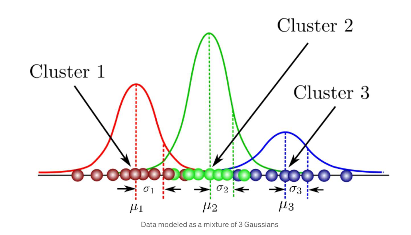
Gaussian Mixture Model (GMM)

• Gaussian Mixture Modelling is the method of modelling data as a weighted sum of Gaussians
  • 高斯混合建模是将数据建模为高斯加权和的方法

Algorithm

• The recent history of each pixel is modeled by a mixture of K Gaussian distributions
• The probability of observing the current pixel value is

\[P(X_t) = \sum_{i=1}^{K} \omega_{i,t} * \eta(X_t, \mu_{i,t}, \Sigma_{i,t})\] \[\eta(X_t,\mu,\Sigma) = \frac{1}{(2\pi)^{\frac{n}{2}} |\Sigma|^{\frac{1}{2}}} e^{-\frac{1}{2}(X_t - \mu_t)^T \Sigma^{-1} (X_t - \mu_t)}\] \[\Sigma_{k,t} = \sigma_k^2 I\]

• To speed up the algorithm
  • K is between 3 and 5
  • The covariance matrix is simplified as a diagonal matrix
  • This assumes that the red, green, and blue pixel values are independent and have the same variances

GMM Algorithm: no match

• If none of the K distributions match the current pixel value, the least probable distribution is replaced with a distribution with the current value as its mean value, an initially high variance, and low prior weight.
• The prior weights of the K distributions at time t, $\omega_{k,t}$, are adjusted as follows:

\[\omega_{k,t} = (1 - \alpha) \omega_{k,t-1} + \alpha(M_{k,t})\]

GMM algorithm: matched pixel value

• The parameters of the distribution which matches the new observation are updated as follows:

\[\mu_t = (1 - \rho)\mu_{t-1} + \rho X_t\] \[\sigma^2_t = (1 - \rho)\sigma^2_{t-1} + \rho(X_t - \mu_t)^{T}(X_t - \mu_t)\]

where

\[\rho = \alpha \eta(X_t | \mu_k, \sigma_k)\]

Tracking targets

• We have seen basic methods to detect change in videos
• We are now going to study methods used to track individual targets, groups and crowds
• There are many tracking algorithms, the most popular include
  • Standard Kalman (Gaussian linear)
    • 标准卡尔曼
  • Extended Kalman (Gaussian non-linear)
    • 扩展卡尔曼
  • Monte Carlo methods such as Condensation (non-Gaussian and non-linear)
    • 蒙特卡洛
  • Hill-climbing posterior, such as the Mean-Shift
    • 爬山后验，如均值漂移

The α − β tracker

简单方法

• Initialisation
  • Set the initial values of state estimates $x$ and $\nu$, using prior information or additional measurements; otherwise, set the initial state values to zero.
  • Select values of the alpha and beta correction gains.
    • 矫正增益数值
• Update - Repeat for each time step $\Delta T$
  • Project state estimates $x$ and $\nu$ using
  • Obtain a current measurement of the output value
  • Compute the residual $r$ 残差
  • Correct the state estimates
  • Send updated $x$ and optionally $\nu$ as the filter outputs

Update phase

• Project state estimates $\hat{x}$ and $v$ using

  \[\hat{x}_k \leftarrow \hat{x}_{k-1} + \Delta T \, \hat{v}_{k-1}\]

\[\hat{v}_k \leftarrow \hat{v}_{k-1}\]

• Obtain a current measurement of the output value $x_k$

• Compute the residual $r$

\[\hat{r}_k \leftarrow x_k - \hat{x}_k\]

• Correct the state estimates

  \[\hat{x}_k \leftarrow \hat{x}_k + (\alpha) \hat{r}_k\] \[\hat{v}_k \leftarrow \hat{v}_k + \left(\frac{\beta}{[\Delta T]}\right) \hat{r}_k\]

• Send updated $x$ and optionally $\nu$ as the filter outputs

Notes

• The corrections can be considered small steps along an estimate of the gradient direction
• As these adjustments accumulate, error in the state estimates is reduced
• For convergence and stability, the values of the alpha and beta multipliers should be positive and small
• Noise is suppressed only if $0 < \beta < 1$ otherwise the noise is amplified

\[{0 < \alpha < 1 ,\\ 0 < \beta \leq 2 ,\\ 0 < 4 - 2\alpha - \beta }\]

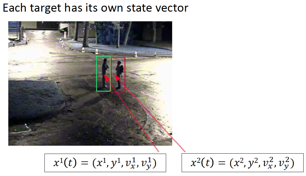
State vector

• One can use position and velocity
• If an object has a 2D shape, we can add width and height of the bounding rectangle

Kalman filter

• The idea is that Kalman helps describing a dynamic system
• The descriptor is a state vector
  • Minimum data sufficient to uniquely describe the dynamics of the system
• The system is continuously updated
  • This is done by using new observations and integrating new information in the model/descriptor
• A target at a given frame t, has an $(x, y)$ position and a $(v_x, v_y)$ velocity
• The Kalman filter predicts the object velocity, given its previous position and a model that keeps on updating

Kalman1960.pdf

Kalman life cycle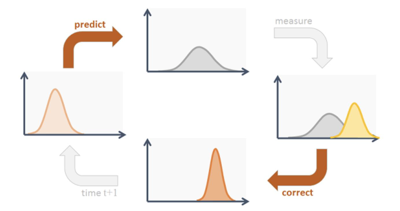

Multi-target complexity and applications

Staged outdoors

Real/Natural outdoors

Multi-target tracking

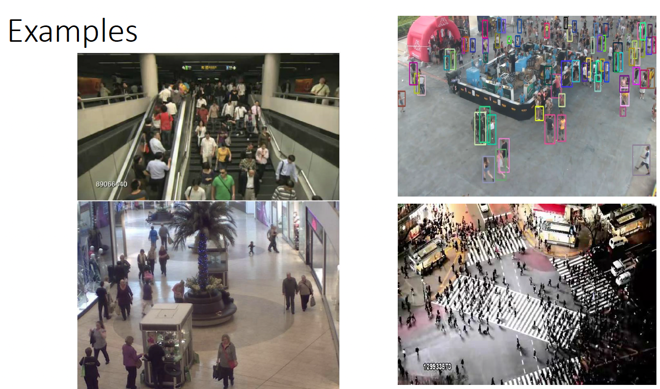
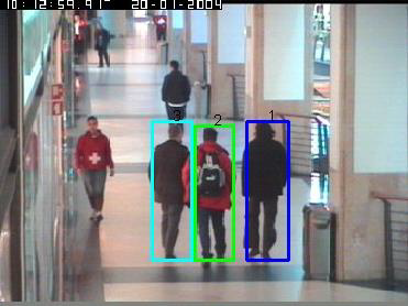
Tracking multiple targets

• Imaging you want to track people in a very cluttered and crowded environment
  • Imagine a shopping mall or an airport
• Even if a security guard seeds the tracking for all the targets, you must develop an algorithm that works when
  • People are only partially visible, targets might disappear for periods of time either behind other people or the environment, say a wall
  • Targets might meet, say shake hands, then occlude one another and then depart in directions different from the original ones
  • People might take off their hat, jumper, or put them on
    etc. …

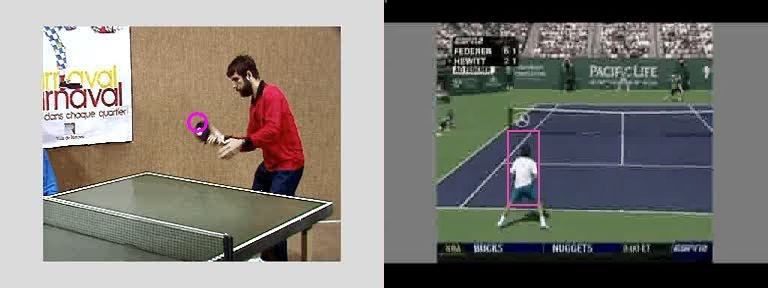
Using particles to follow targets

• We can use very simple modules, we call them particles for each target
• The particles act as a swarm of insects that stick to each other and at the same time follow the target
• We can do this for each target
• The idea is that if some particles get lost because of clutter or unexpected dynamics, some will be able to stick to the target, making it harder for the target to be lost

Particle Swarm Optimisation (PSO) 粒子群优化

• PSO is a population-based optimisation technique
• A set of particles ${x^i}_{i=1}^N$ iteratively find the optimum solution in a search space (for instance the position and velocity space)
• Each particle is a candidate solution equivalent to a point in a $d$-dimensional space, so the $i$th candidate can be represented as $x^i = (x^i_1, x^i_2, x^i_3, \cdots, x^i_d)$
• The movement of each particle depends on two important factors
  • $x^i_b$ the best position that the $i$th candidate has found so far and
  • $x_g$ the global best position found by the whole swarm (all particles)

Updating equations

• Based on these two factors, each candidate updates its velocity and position in the $(n + 1)^{th}$ iteration are as follows

\[v^i(n + 1) = \omega v^i(n) + \varphi_1 r_1 (x^i_b - x^i_n) + \varphi_2 r_2 (x_g - x^i_n)\] \[x^i(n + 1) = x^i(n) + v^i(n + 1)\]

• Where $\omega$ is the inertia weight, the parameters $\varphi_1$ and $\varphi_2$ are positive constants, which balance the influence of the individual best and the global best position.
• The parameters, $r_1, r_2 \in (0,1)$ are uniformly distributed random numbers.

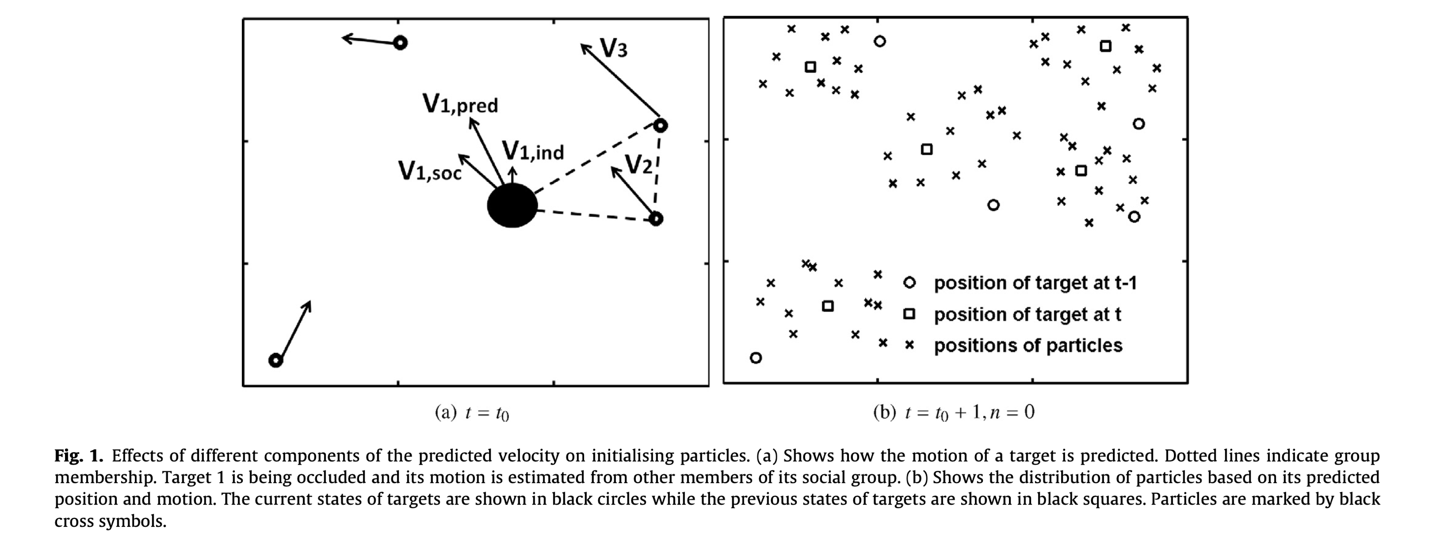
PSO for multiple targets

• Particle Swarm Optimisation (PSO) is based on social behaviour
• We can extend the standard PSO to the problem of multi-target tracking
  • Introduce an idea of multiple interactive swarms
  • Incorporate constraints such as motion information, temporal continuity

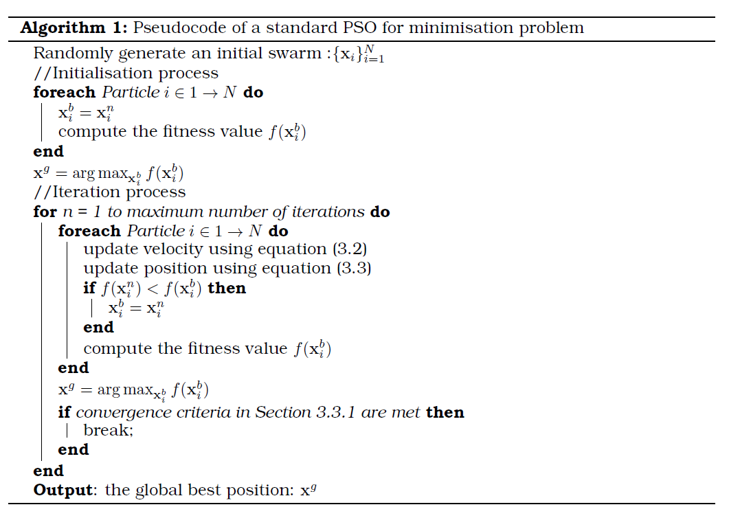
PSO algorithm

PSO combines both the social interaction, individual knowledge

What to optimise?

• Fitness function: evaluating how close each individual particle is from the target

Multi-targets Tracking : PSO vs Multiple swarms

\[v_i^{n+1} = \omega v_i^n + \phi_1 r_1(x_i^b - x_i^n) + \phi_2 r_2(x_g^n - x_i^n)\] \[x_i^{n+1} = x_i^n + v_i^{n+1}\] \[v_i^{n+1} = \chi (v_i^n + \phi_1 r_1(x_i^b - x_i^n) + \phi_2 r_2(x_g^n - x_i^n))\]

where $\chi < 1$ is defined as:

\[\chi = \frac{2}{\parallel 2 - \phi - \sqrt{\phi^2 - 4\phi \parallel }}, \quad \text{where } \phi = (\phi_1 + \phi_2) > 4.0\]

Multiple PSO

• Parameters are assigned based on motion information among swarms
• Motion is predicted based on social information among targets moving in the same direction

\[v_{i,k}^{n+1} = \chi [v_{i,k}^n + c_1 r_1 (x_i^b - x_{i,k}^n) + c_2 r_2 (x_k^g - x_{i,k}^n) + c_3 r_3 (x_k^d - x_{i,k}^n)]\] \[x_{i,k}^{n+1} = x_{i,k}^n + v_{i,k}^{n+1}\]

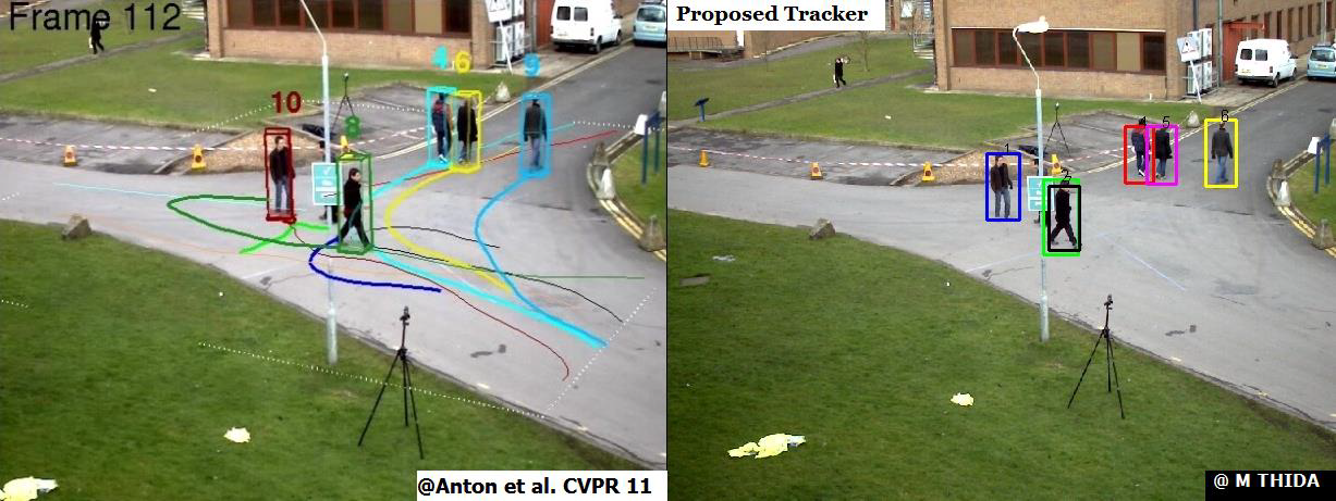
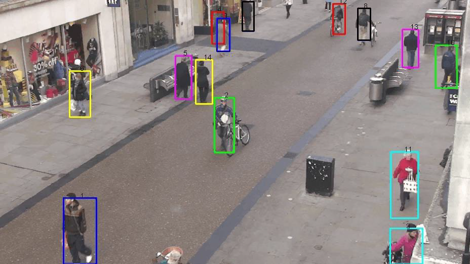
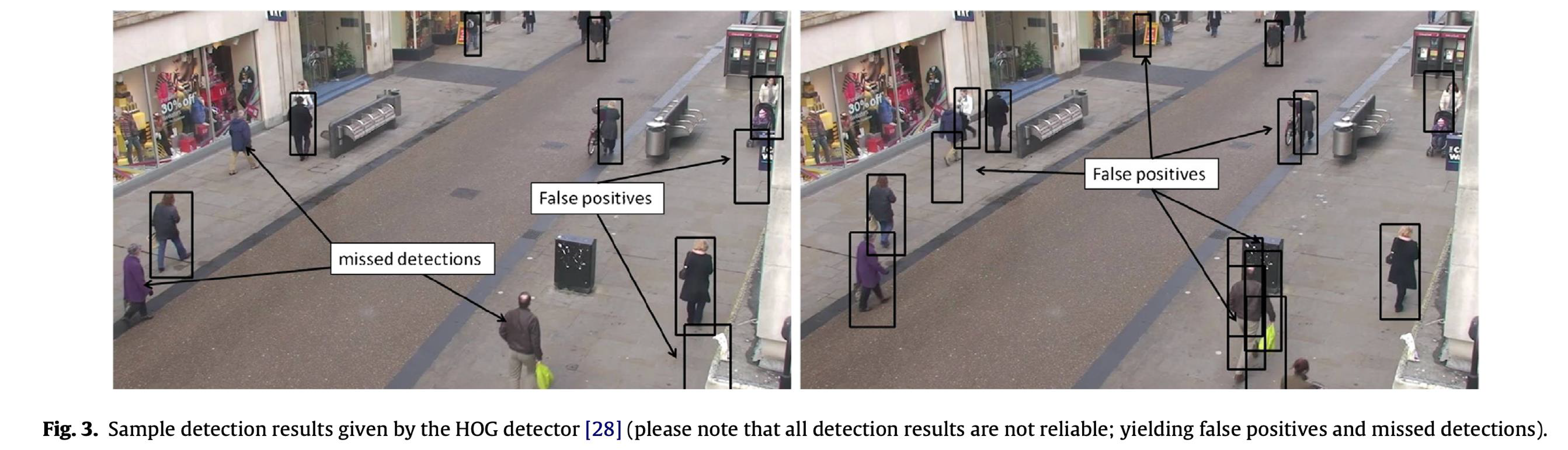
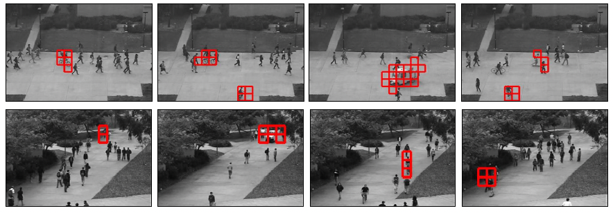
Using HOG to detect targets

• For each frame we use the histograms of oriented gradients (HOG) human detector
• Fig. 3 shows the results of HOG detector in a scene. Please note that all detection results are not reliable; yielding false positives and missed detections.

Guiding the particles

• The next step is to identify a detection response to guide the tracker to a particular target
• Results at time t are provided by t

• the matching score between HOG results and the current state of the tracked target k is based on the spatial proximity, size and the appearance similarity, using

  \[A(x_k, x_m) = A_s(x_k, x_m) \times A_f(x_k, x_m) \times A_d(x_k, x_m)\]
• $A_s$ is the overlapping area between targets k and the detection m
• $A_f$ uses the Bhattacharyya distance between HOG histograms
• $A_d$ is computed using the Euclidean distance between centroid locations of the tracked target k and the detection response m

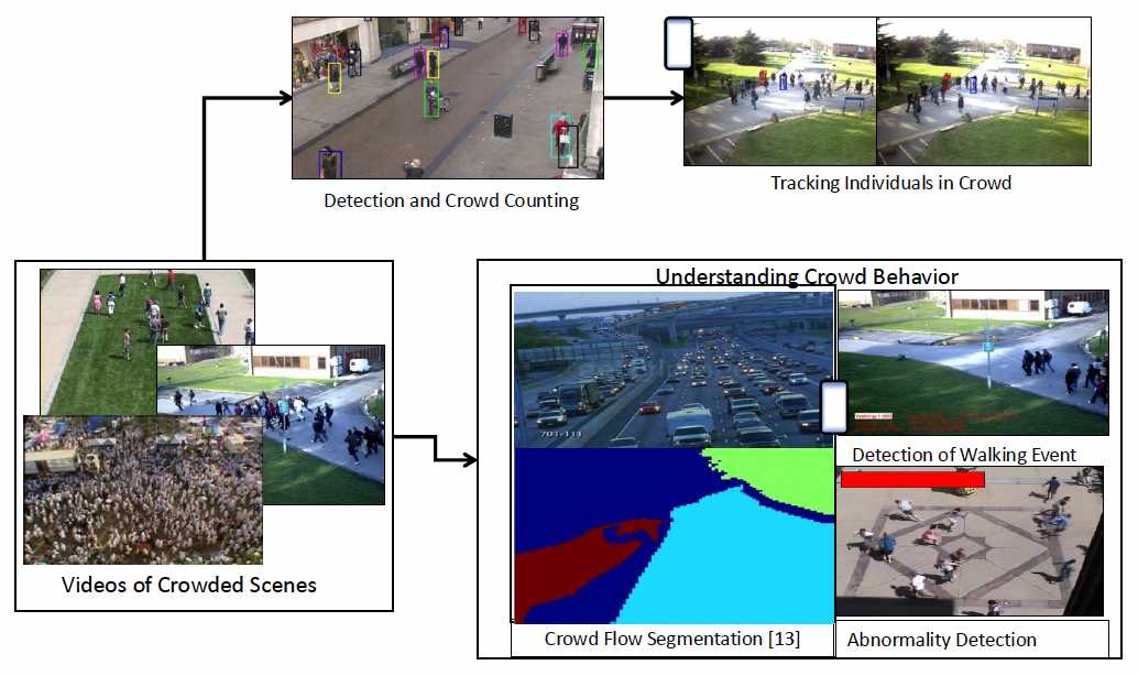
Abnormality Detection and Localization in Crowded Scenes

INTRODUCTION

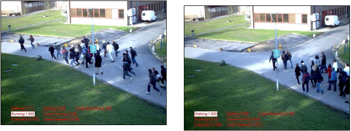
• What is an abnormal event in crowded scene?
  • unusual, rare, atypical, suspicious or outlier.
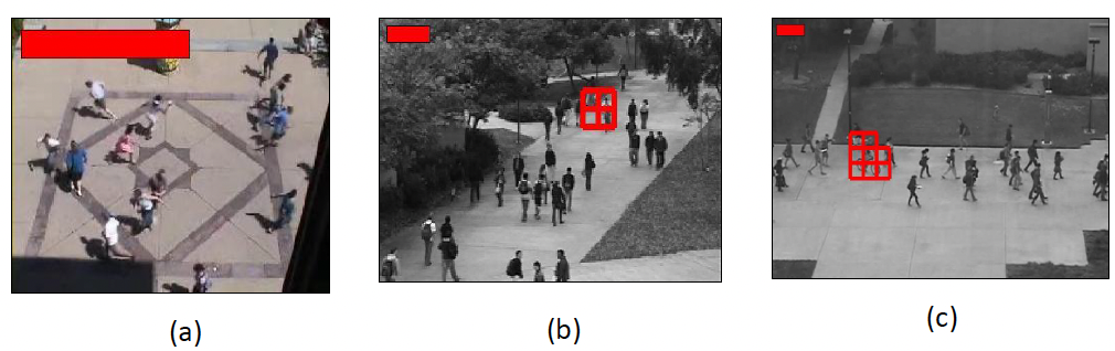
• Two types of abnormality:
  • Global abnormality: most people in the scene move suddenly from the regular behavior (a)
  • Local abnormality: usually arises due to the action of an individual or a group in a crowd (b, c)
• Challenges
  • Localized abnormal behavior
  • Unstructured crowded scenes:
    1. the crowd moves randomly
    2. the crowd direction and density varies over time

PROPOSED METHOD

• To detect and localize abnormal activities in crowded scenes
  • detect not only in global context but also in local context
  • localize the abnormal regions accurately
  • without detecting and tracking individuals
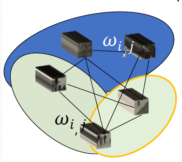
• Video representation: as a fully connected graph G(V;E) where V is a set of local regions and E is a set of edges representing the connectivity between local regions
• Low-dimensional representation: embeds video into a low dimensional space using a Temporally Constrained Laplacian Eigenmap.
• Motion pattern representation: represent the normal behavior as a mixture of Gaussian.
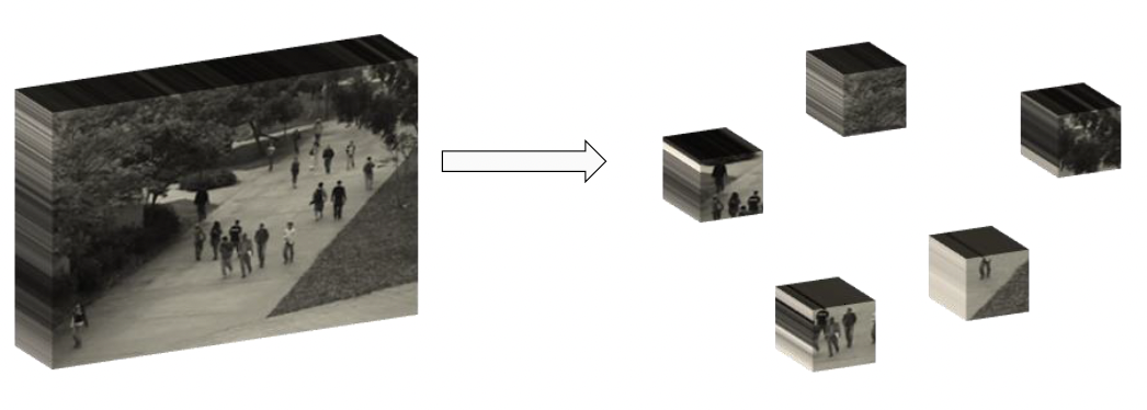
• Video Representation
  • Segment video into clips
  • Subdivide each clip into a set of non-overlapping cubes
  • Represents optical flow vectors in each patch as a weighted histogram
  • Concatenates histograms at each location over T frames

\[x_i = h_{1:T} = [h_1, h_2, \cdots, h_T]\]

• Temporally Constrained Laplacian Eigenmap
  • Computes a pair-wise graph using motion information from local-patches where an edge between two local regions is weighted by
  • Embeds local motion patches into a low-dimensional space
  • Group the embedded-data into K clusters using a k-means clustering method

\[w_{ij} = \exp\left(-\frac{d_{f}^{i,j}}{\sigma_{t}^{i} * \sigma_{t}^{j}}\right) \cdot \exp\left(-\frac{d_{s}^{i,j}}{\sigma_{s}}\right)\]

where $d_{f}^{i,j}$ gives the feature distance and $d_{s}^{i,j}$ gives the spatial distance between two local motions $x_i$ and $x_j$. The sigma values, $\sigma_{i}^{t}$ and $\sigma_{j}^{t}$ are defined as temporally constrained local variances at $r_i$ and $r_j$ respectively.

Motion Pattern Representation

• Represents the regular behavior as a mixture of Gaussian components
  • each group is represented as a single Gaussian:

\[\mu_k = \frac{1}{N_k} \sum_{i=1}^{N_k} x_i, \quad \sigma_k = \frac{1}{N_k} \sum_{i=1}^{N_k} (x_i - \mu_k)^2,\]

and $N_k$ is the total number of data points belonging to the $k^{th}$ group.

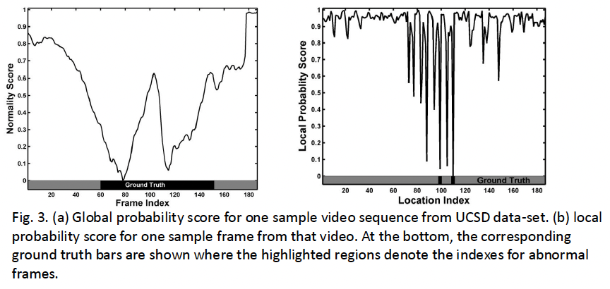
Abnormality detection and localization

Given an unseen sequence, motion pattern is computed

• The normality score for each local region is

  \[p(x_i^{new} | normality) = \sum_{k=1}^{K} \omega_{k,i} \cdot \frac{1}{\sigma_k \sqrt{2\pi}} \exp \left(-\frac{(x_i^{new} - \mu_k)^2}{2\sigma_k^2}\right),\]

  where $\omega_{k,i}$ is the weight of the $k^{th}$ behavior pattern.

• Each location is computed separately

  \[\omega_{k,i} = \frac{n_{k,i}}{\sum_{\epsilon} n_{\epsilon,i}}, \text{ where } \epsilon = \{1, 2, \ldots, K\}\]

  and $n_{k,i}$ is the total number of times activity $k$ occurs at region $i$ while $K$ is the total number of activity patterns.

Proposed Method-cont:

• Abnormality detection and localization
  • Abnormality score for each video frame is computed as:
  \[g(x^{new}|normality) = \frac{1}{N} \sum_{i=1}^{N} p(x^{new}_{i}|normality),\]

  where $N$ is the total number of local regions in each frame.

  • When a frame is detected as abnormal, we then localize the abnormal region
    • the regions with low normality scores are most highly likely to be abnormal.

Experimental Results

• Global Abnormality Detection

  • UMC video data-set [1] is used.

  • 11 video sequences of 3 different scenarios.

  • Each sequence contains a normal starting section and abnormal ending section and has a frame size of 320 by 240.

  • Training set: randomly selected images from the normal starting section

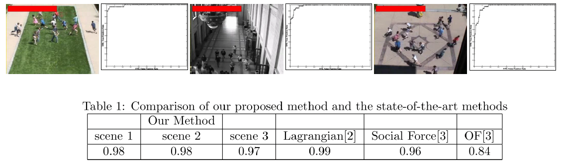
Experimental Results

• Local Abnormality Detection
  • UCSD crowd data-set [4]
    • 98 video sequences from two different scenarios (ped1: frame size 238158 and ped2: frame size 360240)
    • Training set: 50 sequences (34 from ped1 and 16 from ped2)
    • Testing set: 48 sequences (36 from ped1 and 12 from ped2)

Abnormality detector

• Detection and localization of unusual behaviour of an individual or crowd
• Two manifold algorithms based on the Laplacian Eigenmaps to discover internal structure of videos in embedded space
  • Incorporate spatial temporal information
  • Segment a video trajectory
  • Detect abnormal behaviour
• Model the normal behaviour of a crowded scene based on the information in the embedded space
  • Detect and localise abnormal regions (higher accuracy with low computational time)

Group behaviour: fish tank application

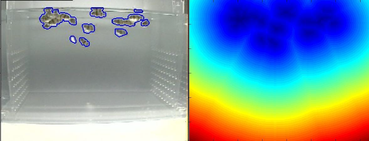
• All drinking water in Singapore is provided by its neighbouring country Malaysia
• There is no trust in the quality of transferred water
• Scientists have devised a method to test it
• A fish tank works as a buffer zone, where the behaviour of fish is recorded and automatically analysed

Problem and Challenges

• Automatic analysis of group behaviour with a countable number of targets
• vision-based analysis of living organisms in the research area of biology and medicine
• Challenges:
  • unpredictable nature of targets in a confined area, no scene layout
  • Movements are random and confined in a small area

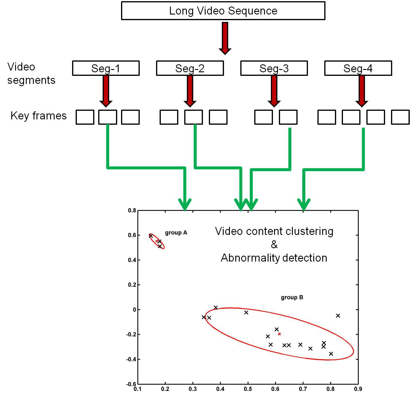
Group behaviour analysis

• Divide long video into short segments
  • Standard approach: sliding window with a fixed scale
  • Proposed: divide by studying the motion and appearance variation
• Key frame extraction
  • Proposed: spectral clustering
• Video Content Clustering and abnormality Detection

Spectral clustering

• Given a set of data points, the first step of spectral clustering is to compute a pairwise similarity matrix W where $w_{ij}$ represents similarity measure between data points $i$ and $j$
• One of the most popular methods is to use Gaussian similarity function

\[w_{ij} = \exp \left\{ -\frac{\| d(i,j) \|^2}{2\sigma^2} \right\}\]

• where $d_{ij}$ is distance measure between two data points and $\sigma$ is a scaling parameter
• A graph Laplacian matrix is computed using the similarity matrix W
• In the method that is described, the following is used

\[L = I - D^{-1/2}WD^{-1/2}\]

• where I is identity matrix, W is similarity matrix
• D is diagonal matrix with values $d_{ii}$ defined as

\[d_{ii} = \sum_{j} w_{ij}\]

• The eigen-decomposition of L is obtained using singular value decomposition
• Data are then clustered using the eigenvalues and corresponding eigenvectors

Algorithm – initial step

• Compute distance measure between all images in an image batch using a suitable distance measure (they included shape)
• The Laplacian matrix is then calculated
• The first K smallest eigenvalues and corresponding eigenvectors are extracted
• K-means clustering is used on the extracted eigenvectors to group the shapes into K clusters
• Representative swimming pattern is extracted

Algorithm - incremental step

For a new image frame

• Compute distance measures between new image and cluster representatives and select the minimum distance
• When a new image is distant from the current representatives, it is added to a set of cluster-to-be
• Spectral clustering is only used when the set of cluster-to-be has sufficient amount of data.
  • This reduces computational cost significantly
• Then, new cluster representatives are augmented into the previous cluster lists

Summary

• We have learned about detection and tracking
• In particular, we have revisited the change detection algorithm
• We have then covered Kalman, Condensation and particle filtering
• We have learnt about abnormality detection and a peculiar application to fish trajectories