CV Lecture 6

CV Lecture 6

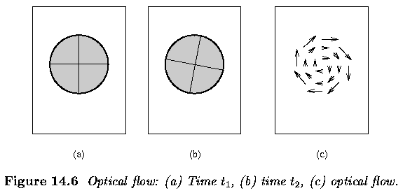
Motion field and the Optical flow

• The Motion Field is the projection of the 3D scene motion into the image
• Optical flow is the apparent motion of brightness patterns in the image
• Ideally, they are the same, but this is not the case all the time

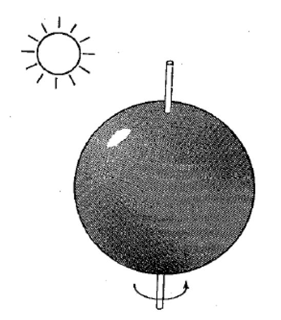
Apparent motion is not the motion field

• Apparent motion can be caused by lighting changes without any actual motion
• For instance, consider a uniform rotating sphere under fixed lighting versus a stationary sphere under moving illumination

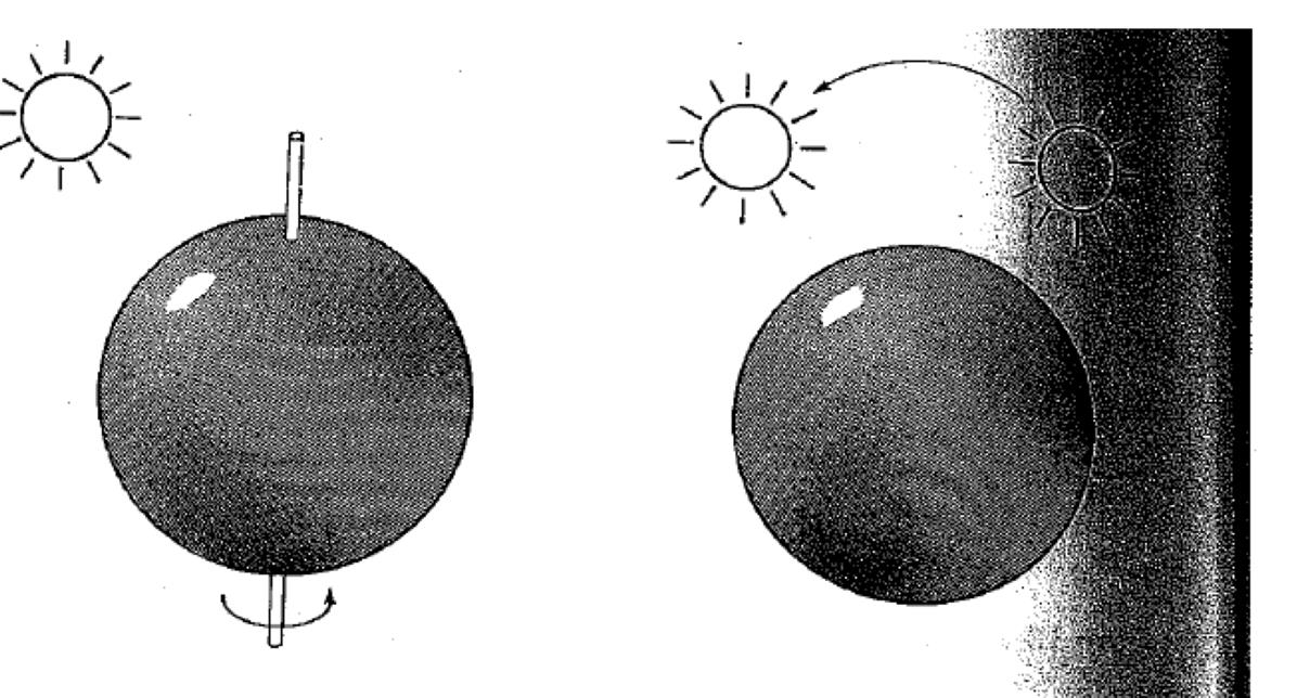
Apparent motion continued

• Apparent motion can be caused by lighting changes without any actual motion
• For instance, consider a uniform rotating sphere under fixed lighting versus a stationary sphere under moving illumination

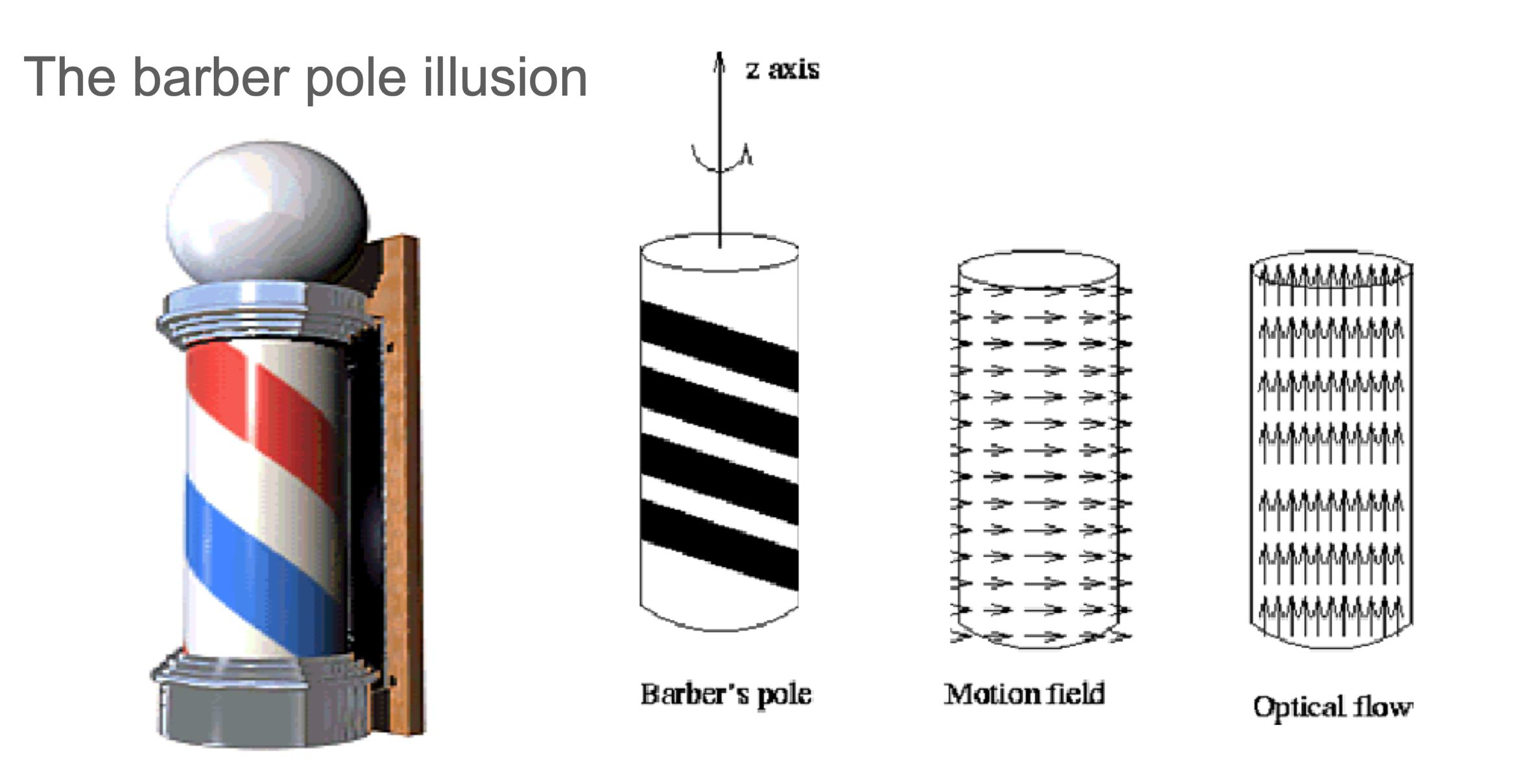
The barberpole illusion

• This visual illusion occurs when a diagonally striped pole is rotated around its vertical axis (horizontally).
• It appears as though the stripes are moving in the direction of its vertical axis (downwards in the case of the animation to the left) rather than around it.

Optical flow (OF)

• Distribution of apparent motion (velocities) of brightness patterns in an image or video sequence
• OF arises from relative motion of objects and the viewer
• It can therefore provide important information about spatial arrangement of the objects captured by the camera
• Each pixel in an image is assigned a velocity vector
• Represents the direction and speed of apparent motion

Why do we need OF?

• Correct camera jitter (stabilization)
• Align images (mosaics)
• 3D shape reconstruction
• Track object behaviour

What is OF?

• Reflects the image changes due to motion during a time interval ( dt ), which is short enough to guarantee small inter-frame motion changes.
• The immediate objective of optical flow is to determine a velocity field.
  • A ( 2D ) representation of a (generally) ( 3D ) motion is called a motion field (velocity field).
  • Whereas each point is assigned a velocity vector corresponding the motion direction, velocity and distance from an observer at an appropriate image location.

OF assumptions

• Based on 2 assumptions
  • The observed brightness of any object point is constant over time
  • Nearby points in the image plane move in a similar manner (velocity smoothness constraint)
• Motion field is a projection of ‘real’ motion vectors of 3D objects to the image plane
• We can only compute an optical flow from time-varying brightness of a given image sequence
• This is an approximation of the motion field

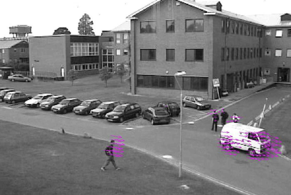
Examples

Pixel based flow estimation

• Estimation
  • Assign a flow vector to each pixel of the changing scene
    • 为变化场景的每个像素分配一个流向量
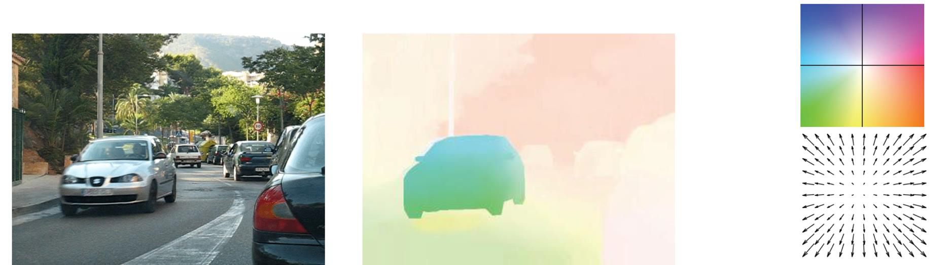
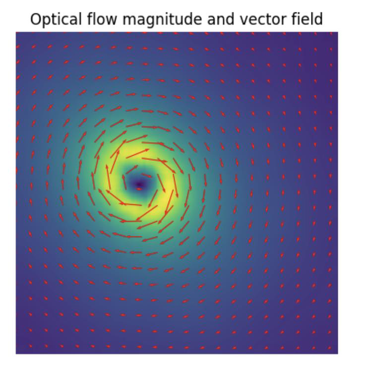
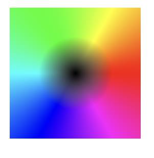
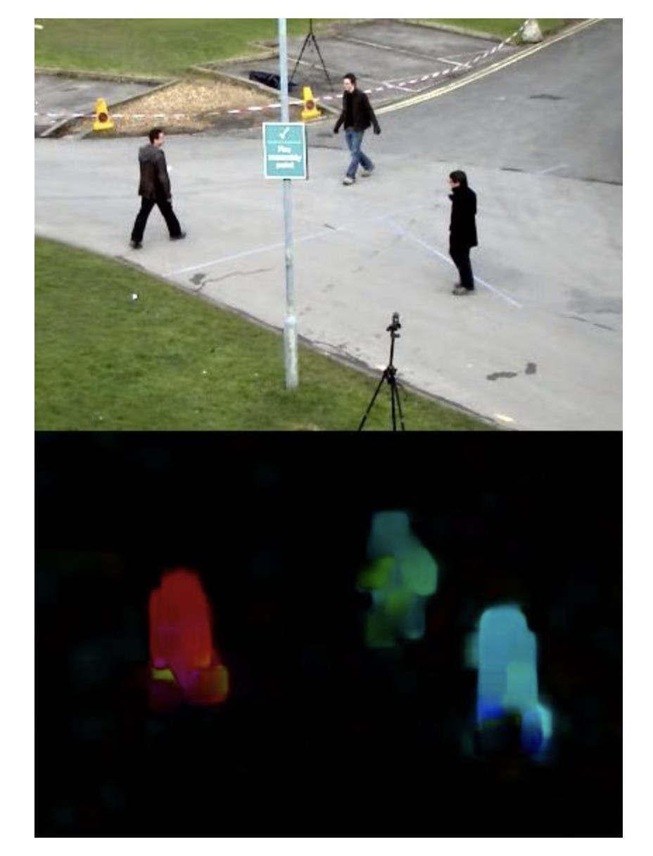
• Visualisation
  • You display the flow, for instance, as flow magnitude (saturation) and orientation (hue)
    • 作为流量大小（饱和度）和方向（色调）

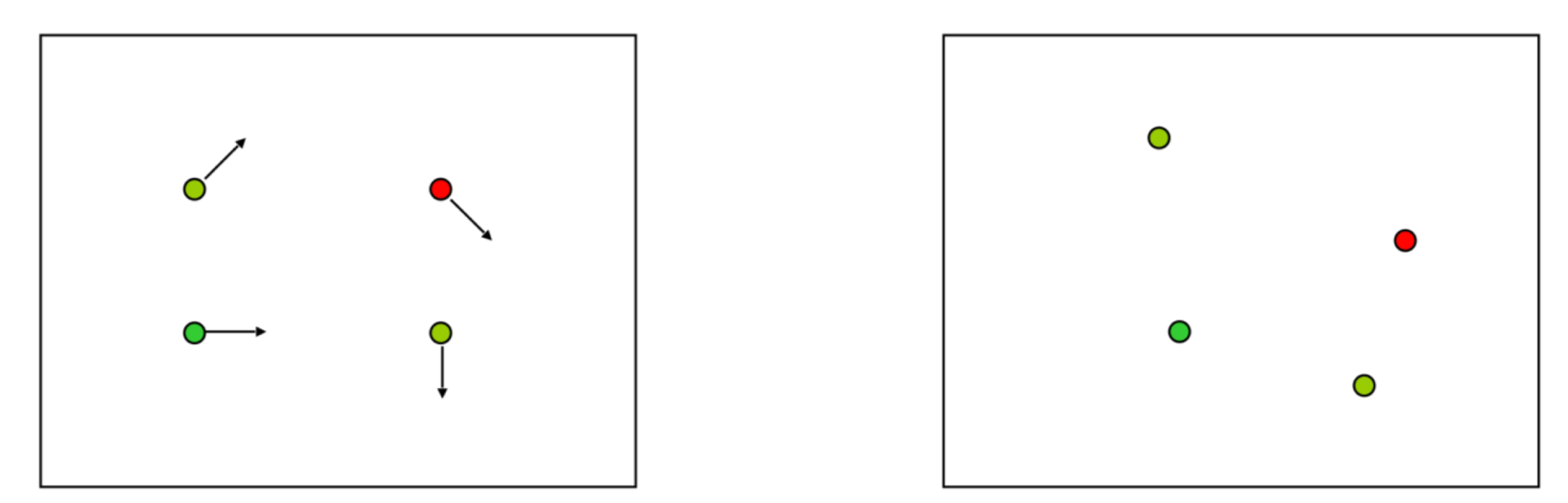
Examples of motion fields

How can we estimate motion?

• Imagine you have two consecutive frames in a sequence
• How can we estimate pixel motion?

Steps

• Given a pixel in the image at time $t, I(x, y, t)$
• For each pixel, we search for pixels nearby in $I(x, y, t + 1)$
• We can then compare, for instance, the colour information
• You will see that we can also use a richer information, such as location and descriptor
  • remember SIFT?
• When we use colour, we make the assumption called
  • Colour or brightness constancy

Optical flow constraint

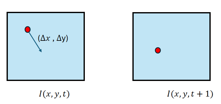
• So, a pixel in $I(x, y, t)$ is displaced by $(\Delta x, \Delta y)$ in the successive frame $I(x, y, t + 1)$
• Brightness constancy implies
  $I(x, y, t) = I(x + \Delta x, y + \Delta y, t + \Delta t)$

Optical flow calculation

• We are making the assumption that a small motion has taken place
• We use the Taylor expansion
  • $I(x + dx, y + dy, t + dt) = I(x,y,t) + I_x(x,y,t)dx + I_y(x,y,t)dy + I_t(x,y,t)dt + \text{error}$
  • We assume the error is roughly zero ((\approx 0))
• So,
  • $I(x,y,t) + I_x(x,y,t)dx + I_y(x,y,t)dy + I_t(x,y,t)dt = 0$

OF calculation continued

We assume that the image does not change given a very short time period, $dt$

\[\begin{aligned} & \frac{dI}{dt}=0 \\ & \Leftrightarrow\frac{dI(x(t),y(t),t)}{dt}=0 \\ & \Leftrightarrow\frac{\partial I}{\partial x}\frac{dx}{dt}+\frac{\partial I}{\partial y}\frac{dy}{dt}+\frac{\partial I}{\partial t}=0 \\ & \Leftrightarrow(\nabla I)^T[\frac{dx}{dt},\frac{dy}{dt}]+I_t=0 \\ & \Leftrightarrow(\nabla I)^T[\frac{dx}{dt},\frac{dy}{dt}]=-I_t \end{aligned}\]

Thus, the displacement vector $\left(\frac{dx}{dt}, \frac{dy}{dt}\right)$ for pixel $(x,y)$ at frame $t$ is the one for which the spatial derivative of the image intensity $I$ at point $(x,y)$ is equal to the negative value of the temporal derivative of $I$ at $(x,y)$.

Check this example

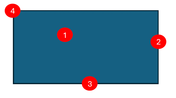
• Imagine you have a rectangle of homogeneous colour
• Imagine we try to estimate motion in a locality of the rectangle
• You have four possibilities, as illustrated in the figure below

What if the rectangle moves

• When it moves
  • Horizontally, 3 and 1 do not change
  • Vertically, 3 and 1 do not change
• So, 4 is the only feature that detects movement whatever the movement of the rectangle might be
• This is why corners are well suited to detect motion

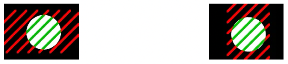
The aperture problem

• Only a component of the motion field in the direction of the spatial image gradient can be computed using the equation

  \[(\nabla I)^T \left[\frac{dx}{dt}, \frac{dy}{dt}\right] = -I_t\]

• This component is called the normal component, because the spatial image gradient is normal to the spatial direction along which the image intensity remains constant.

The motion of a homogeneous contour is locally ambiguous

• This is so because a motion sensor has a finite receptive field: it “looks” at the world through something like an aperture (Hildreth, 1984, 1987)
• Within that aperture, different physical motions are indistinguishable

• In the two given examples, a set of lines moving right to left produce the same spatiotemporal structure as a set of lines moving top to bottom

• The aperture problem implies that motion sensitive neurons in the visual primary cortex will always respond to a contour that crosses their receptive field, independently of its true length and orientation, as long as its direction is consistent with the preferred direction of the neuron
• P. Stumpf is credited with first describing the aperture problem in motion

Computing the displacement vector

• To compute the displacement vector $(dx/dt, dy/dt)$ at pixel $(x,y)$ at frame $t$ we need at least two equations, but at the moment we have only one

\[\begin{bmatrix} \frac{\partial I}{\partial x} & \frac{\partial I}{\partial y} \end{bmatrix}^T \begin{bmatrix} \frac{dx}{dt} \\ \frac{dy}{dt} \end{bmatrix} = -\frac{\partial I}{\partial t}\]

Method 1: we exploit colour

• In colour videos, where we have frames and their three channels: with red R, green G, and blue color intensity values
• This is an overdetermined system
  • We can use least squares, or
  • We ignore one of the equations, say the red channel, and then we use Gauss elimination

\[\begin{bmatrix} \frac{\partial R}{\partial x}, & \frac{\partial R}{\partial y} \end{bmatrix}^T \begin{bmatrix} \frac{dx}{dt}, & \frac{dy}{dt} \end{bmatrix} = -\frac{\partial R}{\partial t}\] \[\begin{bmatrix} \frac{\partial G}{\partial x}, & \frac{\partial G}{\partial y} \end{bmatrix}^T \begin{bmatrix} \frac{dx}{dt}, & \frac{dy}{dt} \end{bmatrix} = -\frac{\partial G}{\partial t}\] \[\begin{bmatrix} \frac{\partial B}{\partial x}, & \frac{\partial B}{\partial y} \end{bmatrix}^T \begin{bmatrix} \frac{dx}{dt}, & \frac{dy}{dt} \end{bmatrix} = -\frac{\partial B}{\partial t}\]

Method 2

• Two assumptions are made
  • Observed brightness of any object point is constant over time
  • Nearby points in the image plane move in a similar manner
    • Velocity smoothness constraint: constant motion vector field in a small patch of the plane

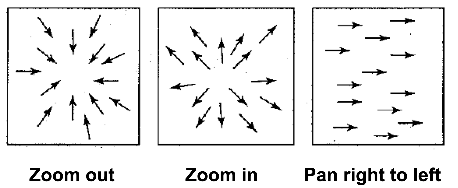
OF in motion analysis

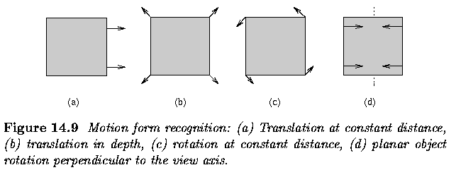
• Motion, as it appears in dynamic images, is usually some combination of 4 basic elements
  • Translation at constant distance from the observer
    • parallel motion vectors
  • Translation in depth relative to the observer
    • Vectors having common focus of expansion
  • Rotation at constant distance from view axis
    • Concentric motion vectors
  • Rotation of planar object perpendicular to the view axis
    • Vectors starting from straight line segments

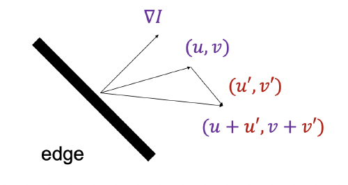
Aperture problem

\[\boxed{I_xu+I_y\nu+I_t=0}\]

Suppose $(u, v)$ satisfies the constraint: $\nabla I \cdot (u, v) + I_t = 0$

• The aperture problem tells us
  Then $\nabla I \cdot (u’ , v + v’) + I_t = 0$ for any $(u’, v’)$ s.t. $\nabla I \cdot (u’, v’) = 0$
  Interpretation: the component of the flow perpendicular to the gradient (i.e., parallel to the edge) cannot be recovered!

Lukas Kanade method

• How to get more equations for a pixel?
• Assumption #3: Spatial coherence constraint.
  assume the pixel’s neighbors have the same (u,v)
  • E.g., if we use a 5x5 window, that gives us 25 equations per pixel

\[\nabla I(x_i) \cdot [u,v] + I_t(x_i) = 0\]

\(\begin{bmatrix} I_x(x_1) & I_y(x_1) \\ I_x(x_2) & I_y(x_2) \\ \vdots & \vdots \\ I_x(x_n) & I_y(x_n) \end{bmatrix} \begin{bmatrix} u \\ v \end{bmatrix} = - \begin{bmatrix} I_t(x_1) \\ I_t(x_2) \\ \vdots \\ I_t(x_n) \end{bmatrix}\)

Lucas Kanade solution

Least squares problem:

\[\begin{bmatrix} I_x(x_1) & I_y(x_1) \\ I_x(x_2) & I_y(x_2) \\ \vdots & \vdots \\ I_x(x_n) & I_y(x_n) \end{bmatrix} \begin{bmatrix} u \\ v \end{bmatrix} = - \begin{bmatrix} I_t(x_1) \\ I_t(x_2) \\ \vdots \\ I_t(x_n) \end{bmatrix}\]

Solution given by \((A^T A)d = A^T b\)

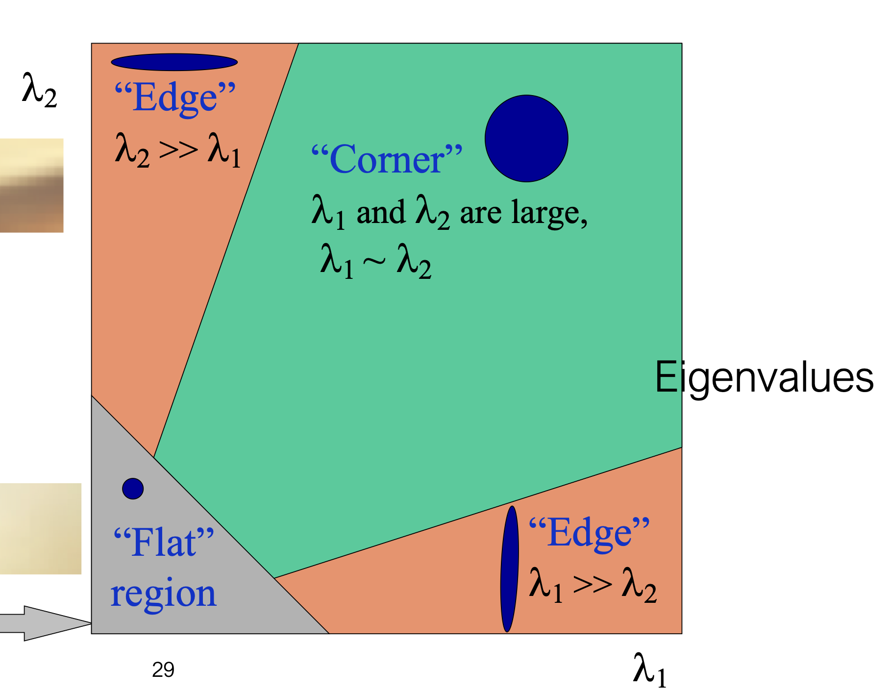
When is this system solvable?

• $M$ must be invertible
• $M$ must be well-conditioned

\(\mathbf{A}_{n\times2}\mathbf{d}_{2\times1}=\mathbf{b}_{n\times1}\) \(M = A^T A \text{ is the “second moment” matrix (also Gauss-Newton approximation to Hessian)}\)

Very similar to Harris corner detector

\[(A^T A)d = A^T b\] \[M = A^T A\]

• M must be invertible
• M must be well-conditioned
• 

How do you display OF

• You can use small vectors

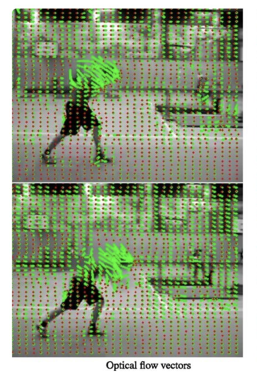
• You can use colours
  • Colour denotes direction of flow at some point
  • Intensity denotes length of displacement vector

Using deep learning methods

The following table compares traditional and modern methods, using deep learning

Algorithm	Accuracy	Speed (FPS)	Computational Requirements
Lucas-Kanade	Moderate	High	Low
Horn-Schunck	High	Low	High
FlowNet	High	Moderate	Moderate
LiteFlowNet	Very High	Moderate	Moderate
PWC-Net	Very High	High	High