CV Lecture 7

CV Lecture 7

Tracking a dynamic system

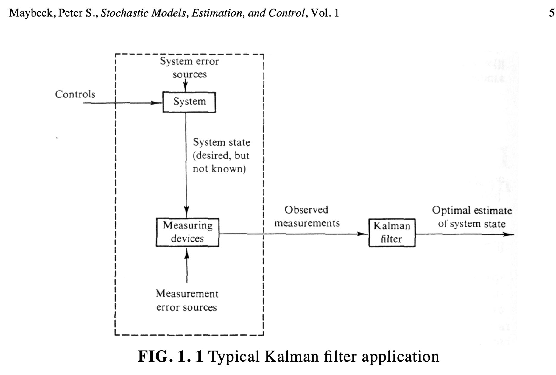
Given a physical system, whether it be an aircraft, a chemical process, or the national economy, an engineer first attempts to develop a mathematical model that adequately represents some aspects of the behavior of that system. Through physical insights, fundamental “laws,” and empirical testing, he tries to establish the interrelationships among certain variables of interest, inputs to the system, and outputs from the system.

We must study our problem, define a system and understand its dynamics

• A system can be anything
  • a video capturing a moving scene is only an example
• A state vector must be used to describe the dynamics
• So, if we had a car that moves across the field of view of a security camera
  • We could represent it with its position and its velocity
  • We would then have a state vector with four values

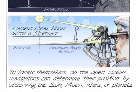
Very simple example: being lost at sea

• You are lost at sea and do not know your current location
• You use the stars to establish your position
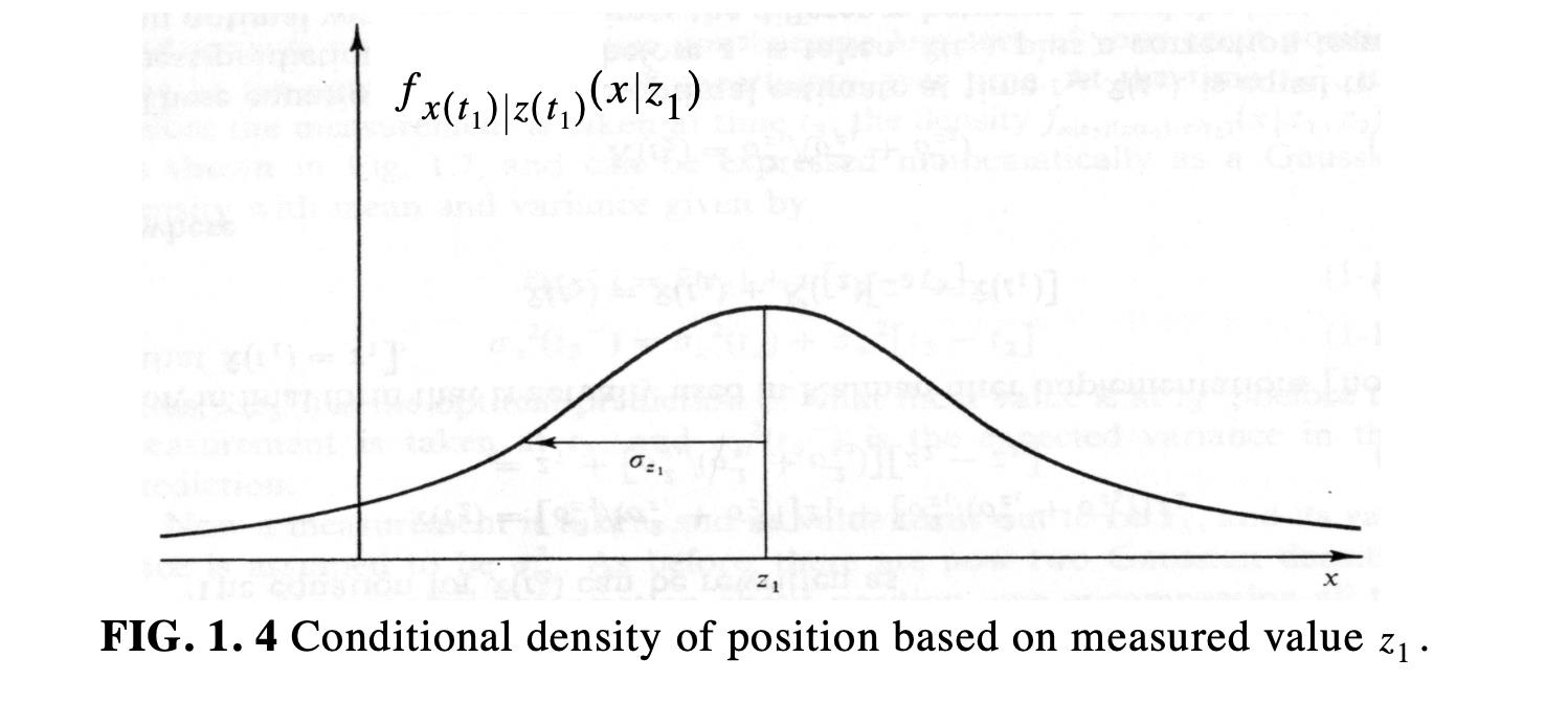
• Say your position is a single value $x$
• So, at time $t_1$ you determine your location with an observation as $z_1$
• Your measurement is inaccurate, so you can assume your estimate has a standard deviation $\sigma_1$

Conditional probability

So

\[\hat{x}(t_1) = z_1\]

and

\(\sigma^2_x(t_1) = \sigma^2_{z_1}\) ### Mean, Variance & Standard Deviation

• (Mean) $\mu = \frac{\sum_{i=1}^{N} x_i}{N}$
• (Variance) $\sigma^2 = \frac{\sum_{i=1}^{N} (x_i - \mu)^2}{N}$
• (Standard Deviation) $\sigma = \sqrt{\frac{\sum_{i=1}^{N} (x_i - \mu)^2}{N}}$
• 

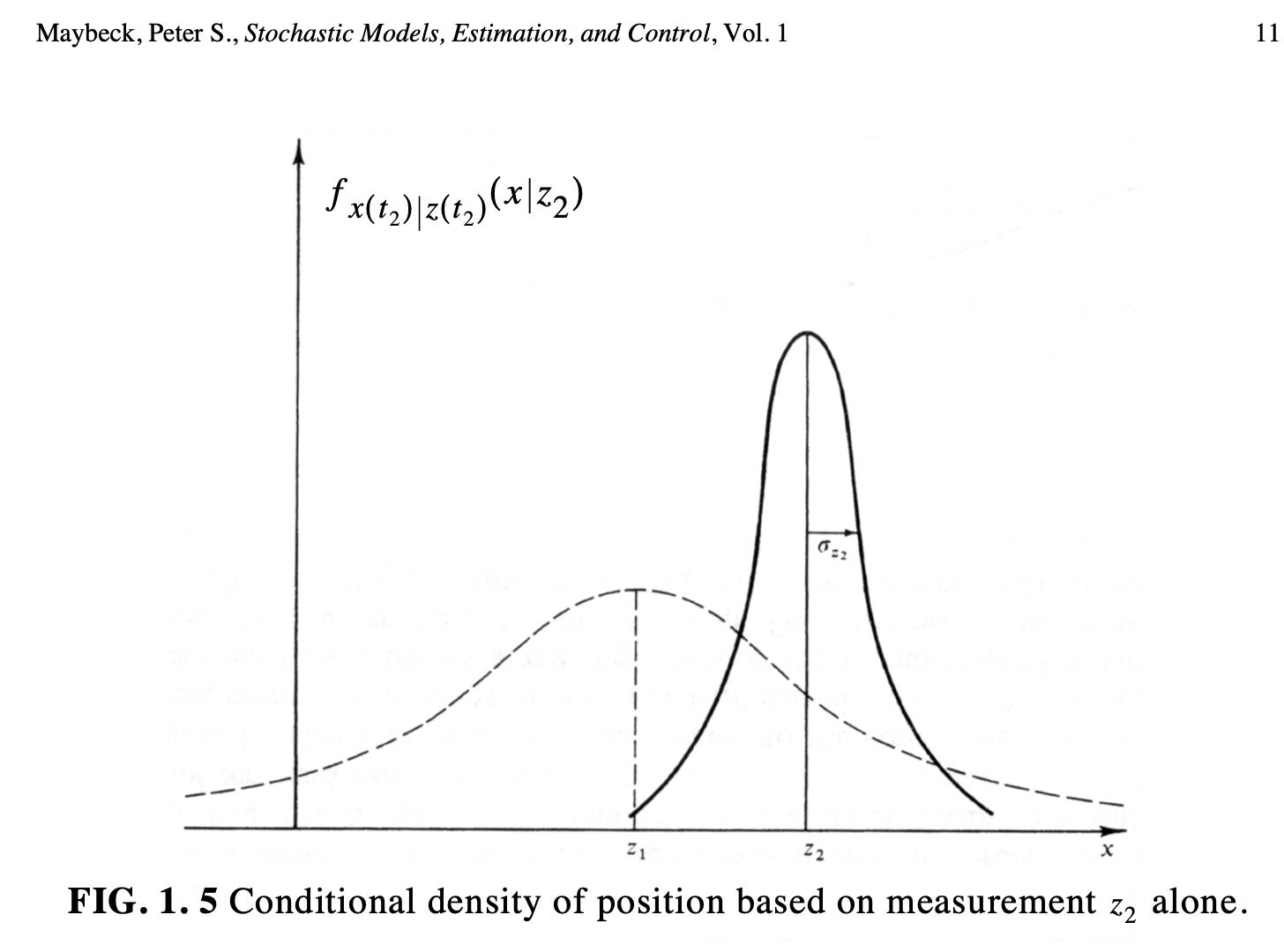
Some help from a friend

• Let us now say that you think your estimate is not good enough
  • … perhaps, you do not feel confident
• So, you ask a friend who is more experienced
• You do this at time $t_2$, one tick ahead
• Your friend does the measurement and obtains $(z_2, \sigma_{z_2})$
• Your friend is more experienced, so you assume that the variance of their observation is more accurate
  • say 1.5 times more accurate

Conditional density after two observations

• You now must combine both observations
• You must take into consideration the standard deviation of both

Combination

\[\begin{aligned} \mu = \left[\frac{\sigma^2_2}{\sigma^2_1 + \sigma^2_2}\right]z_1 + \left[\frac{\sigma^2_1}{\sigma^2_1 + \sigma^2_2}\right]z_2 \\ \frac{1}{\sigma^2} = \left(\frac{1}{\sigma^2_1}\right) + \left(\frac{1}{\sigma^2_2}\right)\end{aligned}\] \[\boxed {f_{x(t_2)|z(t_1), z(t_2)}(x|z_1, z_2)}\]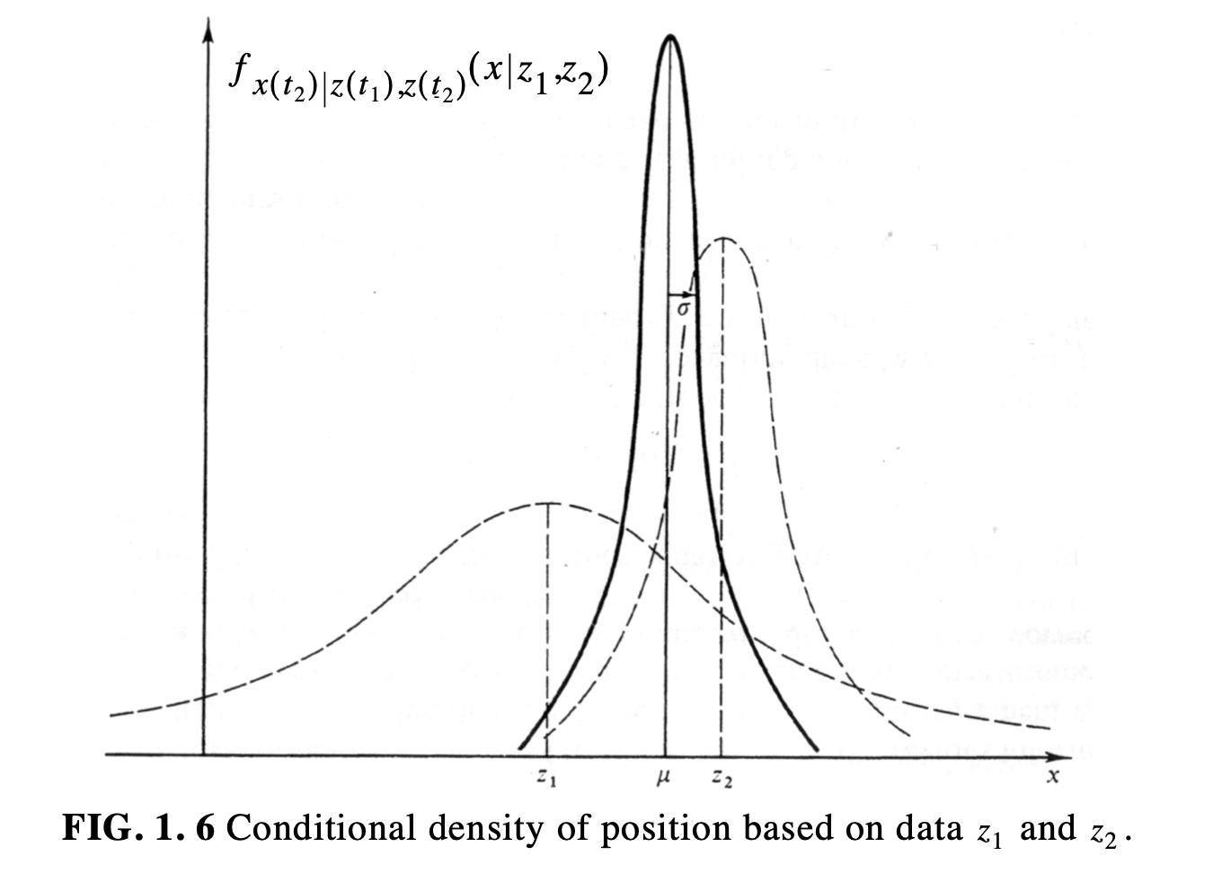

• The combined $\sigma$ is smaller than both $\sigma_{z_1}$ and $\sigma_{z_2}$

Rearranging the equations

• We can now rewrite the equation for $\hat{x}(t_2)$ as follows

\[\hat{x}(t_2) = \left[\frac{\sigma^2_2}{(\sigma^2_1 + \sigma^2_2)}\right]z_1 + \left[\frac{\sigma^2_1}{(\sigma^2_1 + \sigma^2_2)}\right]z_2 = z_1 + \left[\frac{\sigma^2_1}{(\sigma^2_1 + \sigma^2_2)}\right][z_2 - z_1]\]

• Given that $\hat{x}(t_1) = z_1$

\[\hat{x}(t_2) = \hat{x}(t_1) + K(t_2)[z_2 - \hat{x}(t_1)]\]

where

\[K(t_2) = \frac{\sigma^2_1}{(\sigma^2_1 + \sigma^2_2)}\]

In other words

• The two above equations tell us that $\hat{x}(t_2)$, the optimal state at time $t_2$, is equal to the best prediction of its value before $z_2$ is taken, i.e. $\hat{x}(t_1)$, plus a correction term

• We can rewrite the second equation as follows

  \[\sigma^2_{x}(t_2) = \sigma^2_{x}(t_1) - K(t_2)\sigma^2_{x}(t_1)\]

• So, we have solved the estimation problem for a static system

What if you moved

• If you travelled for some time before taking another measurement
  • Then you must take into consideration your speed $dx/dt = u+ w$
  • This will be subject to some noise Gaussian $w$ with variance $\sigma^2_w$

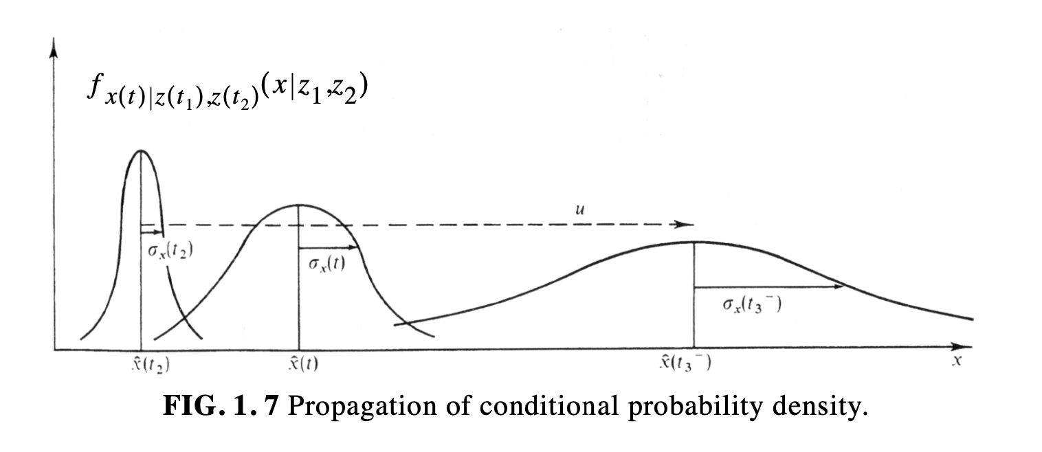
• The probability density moves according to the chosen dynamics and spreads out in time, about its mean
  • This because you become less confident about your exact position
• The time just before the 3rd measurement at $t_3$ can be written as follows

\[\hat{x}(t_3^-) = \hat{x}(t_2) + u[t_3 - t_2]\] \[\sigma^2_x(t_3^-) = \sigma^2_x(t_2) + \sigma^2_w[t_3 - t_2]\]

Thus, $\hat{x}(t_3^-)$ is the optimal prediction of what the $x$ value is at $t_3^-$, before the measurement is taken at $t_3$, and $\sigma^2_x(t_3^-)$ is the expected variance in that prediction.

At time $t_3$

• You take the third measurement $z_3$ and obtain

\[\hat{x}(t_3) = \hat{x}(t_3^-) + K(t_3)[z_3 - \hat{x}(t_3^-)]\] \[\sigma_x^2(t_3) = \sigma_x^2(t_3^-) - K(t_3)\sigma_x^2(t_3^-)\]

where

\[K(t_3) = \frac{\sigma_x^2(t_3^-)}{[\sigma_x^2(t_3^-) + \sigma_z^2(z_3)]}\]

Dynamic scene

• Assume you have a dynamic scene
  • One or more targets can move in the scene
  • For the time being we assume a single fixed camera
  • we assume we have a single target
  • We want to track its projection on the image plane

• At time $t$, the target has a position $p(t)$ and a velocity $v(t)$

• Since we are talking of movement on an image plane
  • The position could be the centroid of the moving object captured by the camera
  • The velocity, its movements in $x$ and $y$ directions, i.e. the two Cartesian axes

Kalman assumptions and goal

• The Kalman filter assumes that
  • both position and velocity can vary
  • Also assumes that the variables are random samples of a Gaussian distribution
  • This means they have mean and variance values
  • Position and velocity are correlated: the likelihood of observing an object at a particular position depends on the velocity of the target
• The last point is the most interesting one as
  • One measurement tells us something about what the future ones could be
  • That is the goal of the Kalman filter

Kalman captures the correlation

• Kalman uses correlation and it uses a covariance matrix as mathematical object
• At time $t$, we have an estimate of the target position $p$, velocity $v$ and their covariance matrix $P$

\[\hat{x} = \begin{bmatrix} p \\ v \end{bmatrix} \quad P = \begin{bmatrix} \sigma_{pp} & \sigma_{pv} \\ \sigma_{vp} & \sigma_{vv} \end{bmatrix}\]

Kalman prediction step

if we assume constant velocity, so no acceleration, then the position of the target will change the following equations

• $p_k = p_{k-1} + \Delta t \cdot v_{k-1}$

and

• $v_k = v_{k-1}$

Kalman covariance updating

• We assume a given time clock tick $\Delta t$

• We now define the state transition matrix $F_k$

  • $$\hat{x}_k=

\begin{bmatrix} 1 & \Delta t
0 & 1 \end{bmatrix}\hat{x}_{k-1}$$ where

\[F_k= \begin{bmatrix} 1 & \Delta t \\ 0 & 1 \end{bmatrix}\]

• So,$\hat{x}k=F_k\hat{x}{k-1}$

• It turns out that the covariance matrix Pk can also be updated using the $F_k$ matrix

  • $P_k = F_k P_{k-1} F_k^T$

External influence

• A dynamic system might also be affected by external forces
• For instance, the software installed on a robot might issue the halting of the robot’s wheels
• … or a drone could be moved by gusts of wind

• We can use $u_k$ as a vector that describes the external influence

• We can add an acceleration $a$ to the system and rewrite the updating equations
  • $p_k = p_{k-1} + \Delta t \, v_{k-1} + \frac{1}{2} a \Delta t^2 = p_{k-1}+\Delta t \cdot v_{k-1}$
  • $v_k = v_{k-1} + a \Delta t$

• We can now rewrite the previous equations in matrix format

  • $$\hat{x}k = F_k \hat{x}{k-1} + \left[ \frac{\Delta t^2}{2} \Big/ \Delta t \right] a

  = F_k \hat{x}_{k-1} + B_k u_k

  $$

  • where $B_k$ is called the control matrix and $u_k$ the control vector

We must include effect of noise

• The covariance updating is incomplete
  $P_k = F_k P_{k-1} F_k^T$

• We must add a covariance matrix that takes noise into consideration
  $P_k = F_k P_{k-1} F_k^T + Q_k$

• We can interpret $Q_k$ as whatever cannot be tracked by the plain state equation

• In other words, the new best estimate is a prediction made from previous best estimate, plus a correction for known external influences

• … and the new uncertainty is predicted from the old uncertainty, with some additional uncertainty from the environment

Kalman: expected transformation

• We can use the matrix $H_k$ to describe the transformation at time step $k$
• This transformation will affect both mean and covariance of the state vector
  • $\hat{\mu}_{exp} = H_k \hat{x}_k$
  • $\Sigma_{exp} = H_k P_{k-1} H_k^T$

Sensor noise

• From each reading we observe, we might guess that our system was in a particular state
• But because there is uncertainty, some states are more likely than others to have have produced the reading we had
• We call the covariance of this uncertainty (i.e. of the sensor noise) $R_k$
• The distribution has a mean equal to the reading we observed, which we call it $z_k$

Two uncertain state vectors

• We have a prediction, following a Gaussian distribution
• We also have a new noisy measurement, provided by the sensor observation
  • This one follows a Gaussian distribution
• We must try to reconcile the predicted state with the observations made with our sensor readings
• This means combining Gaussians

Combining Gaussians

• The solution calls for the combination of two Gaussians.
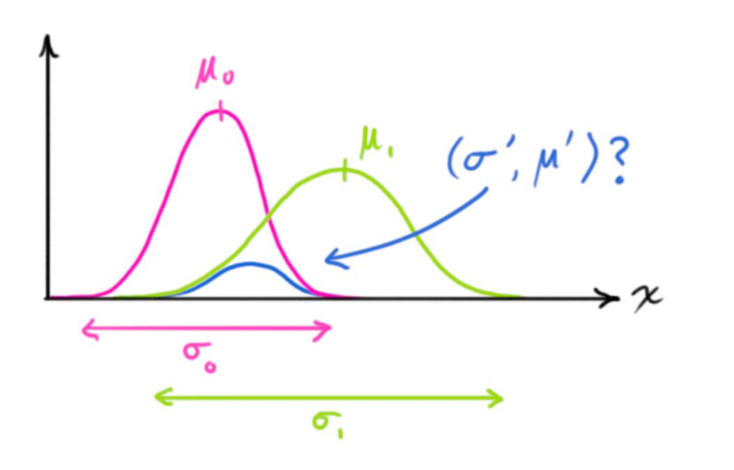
• This cannot be taken lightly, there is a specific way to do it.

• First of all, we define what is called the Kalman gain

  • $K = \Sigma_0(\Sigma_0 + \Sigma_1)^{-1}$

• Then, we can write the two updating equations for the mean vector and related covariance matrix

  • $\mu’ = \mu_0 + K(\mu_1 - \mu_0)$
  • $\Sigma’ = \Sigma_0 - K \Sigma_0$

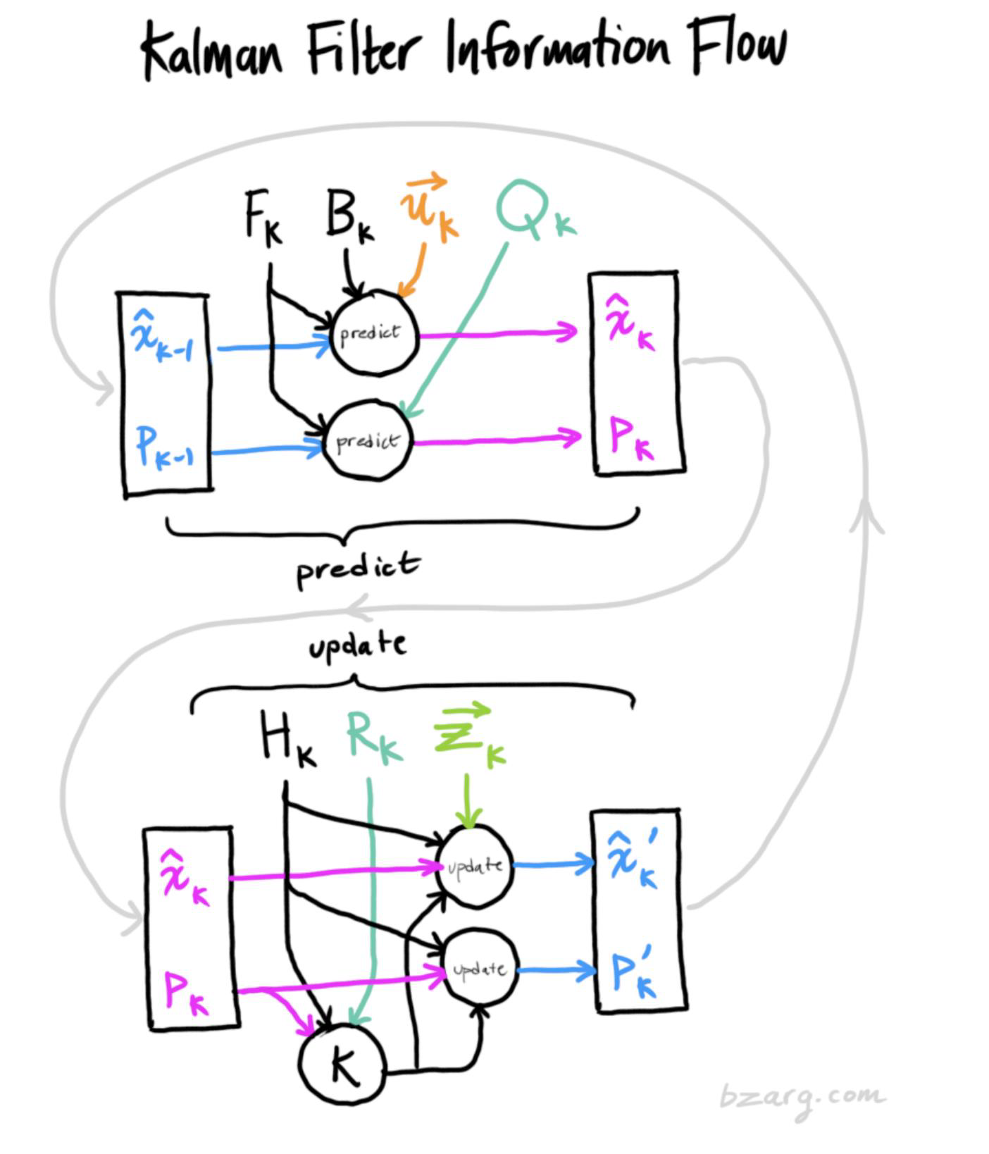
Putting it all together

• We have
  $(\mu_0, \Sigma_0) = (H_k \hat{x}_k, H_k P_k H_k^T) \ \ \ \ \ (\mu_1, \Sigma_1) = (z_k, R_k)$

• After some manipulations, we obtained the final equations
  • Those we saw in my lecture on tracking methods
    $\hat{x}’_k = \hat{x}_k + K’(z_k - H_k \hat{x}_k) \ \ \ \ \ P’_k = P_k - K’ H_k P_k$
• And finally,
  $K’ = P_k H_k^T (H_k P_k H_k^T + R_k)^{-1}$

A simple example

• Let us assume we have an object moving following the equation

  \[f(t) = 0.1 \ast (t^2 - t)\]

• The kinematic equations give us, the updating in position and velocity as follows

  \[x_k = x_{k-1} + \dot{x}_{k-1}\Delta t + \frac{1}{2} \ddot{x}_{k-1}(\Delta t)^2\] \[\dot{x}_k = \dot{x}_{k-1} + \ddot{x}_{k-1}\Delta t\]

Using the matrix formulation

• We can re-write the previous equations in matrix format as follows

  \[x_k = \begin{bmatrix} x_k \\ \dot{x}_k \end{bmatrix} = \begin{bmatrix} x_{k-1} + \dot{x}_{k-1}\Delta t + \frac{1}{2}\ddot{x}_{k-1}\Delta t^2 \\ \dot{x}_{k-1} + \ddot{x}_{k-1}\Delta t \end{bmatrix}\]

• … after some manipulations

  \[x_k = \begin{bmatrix} 1 & \Delta t \\ 0 & 1 \end{bmatrix} x_{k-1} + \begin{bmatrix} \frac{1}{2}(\Delta t)^2 \\ \Delta t \end{bmatrix} \ddot{x}_{k-1}\]

  其中

  \[A = \begin{bmatrix} 1 & \Delta t \\ 0 & 1 \end{bmatrix}\] \[B = \begin{bmatrix} \frac{1}{2}(\Delta t)^2 \\ \Delta t \end{bmatrix}\]

The transformation matrix

• Measurements can be written as
  $z_k = Hx_k + v_k$

• We are only measuring the position, so
  $z_k = \begin{bmatrix} 1 & 0 \end{bmatrix} \begin{bmatrix} x_k \ \dot{x}_k \end{bmatrix} + v_k$

  $H = \begin{bmatrix} 1 & 0 \end{bmatrix}$

Process noise

• The process noise covariance matrix $Q$ or error in the state process can be written as follows

\[Q = \begin{bmatrix} \sigma_x^2 & \sigma_x\sigma_{\dot{x}} \\ \sigma_{\dot{x}}\sigma_x & \sigma_{\dot{x}}^2 \end{bmatrix}\]

• Where $\sigma_x$ and $\sigma_{\dot{x}}$ are the standard deviations of the position and the velocity, respectively

• We can define the standard deviation of position as the standard deviation of acceleration $\sigma_a$ multiplied by $\frac{\Delta t^2}{2}$

• The reason for this is because the $\frac{\Delta t^2}{2}$ is the effect that will have on the position, giving us the standard deviation on position.

… and the measurement noise?

• Similarly, if we multiply the standard deviation of the acceleration by delta $\Delta t$, we get the standard deviation of the velocity.

• So, we can write the process covariance noise $Q$ as follows:

\[Q = \begin{bmatrix} \frac{\Delta t^4}{4} & \frac{\Delta t^3}{2} \\ \frac{\Delta t^3}{2} & \Delta t^2 \end{bmatrix} \sigma_a^2\]

• The covariance of the measurement noise $R$ is a scalar and is equal to the variance of the measurement noise. It can be written as:

\[R = \sigma_z^2\]

A 2D object

• We have just seen how to deal with simple dynamics in one dimension
• Let us make things a bit more complex
  • We can try with dynamics in 2D
• We start from the equations used for the one dimensional case

\[x_k = \begin{bmatrix} x_k \\ \dot{x}_k \end{bmatrix} = \begin{bmatrix} x_{k-1} + \dot{x}_{k-1} \Delta t + \frac{1}{2} \ddot{x}_{k-1} \Delta t^2 \\ \dot{x}_{k-1} + \ddot{x}_{k-1} \Delta t \end{bmatrix}\] \[x_k = \begin{bmatrix} x_k \\ \dot{x}_k \end{bmatrix} = \begin{bmatrix} 1 & \Delta t \\ 0 & 1 \end{bmatrix} \begin{bmatrix} x_{k-1} \\ \dot{x}_{k-1} \end{bmatrix} + \begin{bmatrix} \frac{1}{2} (\Delta t)^2 \\ \Delta t \end{bmatrix} \ddot{x}_{k-1}\]

We then extend to 2D dynamics

• Equations are a bit more complex
• The concept is still the same

\[x_k = \begin{bmatrix} x_k \\ y_k \\ \dot{x}_k \\ \dot{y}_k \end{bmatrix} = \begin{bmatrix} x_{k-1} + \dot{x}_{k-1} \Delta t + \frac{1}{2} \ddot{x}_{k-1} \Delta t^2 \\ y_{k-1} + \dot{y}_{k-1} \Delta t + \frac{1}{2} \ddot{y}_{k-1} \Delta t^2 \\ \Delta t \\ \dot{y}_{k-1} + \ddot{y}_{k-1} \Delta t \end{bmatrix}\] \[\mathbf{x}_k= \begin{bmatrix} x_k \\ y_k \\ \dot{x}_k \\ \dot{y}_k \end{bmatrix}= \begin{bmatrix} 1 & 0 & \Delta t & 0 \\ 0 & 1 & 0 & \Delta t \\ 0 & 0 & 1 & 0 \\ 0 & 0 & 0 & 1 \end{bmatrix} \begin{bmatrix} x_{k-1} \\ y_{k-1} \\ \dot{x}_{k-1} \\ \dot{y}_{k-1} \end{bmatrix}+ \begin{bmatrix} \frac{1}{2}(\Delta t)^2 & 0 \\ 0 & \frac{1}{2}(\Delta t)^2 \\ \Delta t & 0 \\ 0 & \Delta t \end{bmatrix} \begin{bmatrix} \ddot{x}_{k-1} \\ \ddot{y}_{k-1} \end{bmatrix}\] \[x_k = \begin{bmatrix} x_k \\ y_k \\ \dot{x}_k \\ \dot{y}_k \end{bmatrix} = \begin{bmatrix} 1 & 0 & \Delta t & 0 \\ 0 & 1 & 0 & \Delta t \\ 0 & 0 & 1 & 0 \\ 0 & 0 & 0 & 1 \end{bmatrix} x_{k-1} + \begin{bmatrix} \frac{1}{2}(\Delta t)^2 & 0 \\ 0 & \frac{1}{2}(\Delta t)^2 \\ \Delta t & 0 \\ 0 & \Delta t \end{bmatrix} a_{k-1}\] \[A = \begin{bmatrix} 1 & 0 & \Delta t & 0 \\ 0 & 1 & 0 & \Delta t \\ 0 & 0 & 1 & 0 \\ 0 & 0 & 0 & 1 \end{bmatrix} ,\ B = \begin{bmatrix} \frac{1}{2}(\Delta t)^2 & 0 \\ 0 & \frac{1}{2}(\Delta t)^2 \\ \Delta t & 0 \\ 0 & \Delta t \end{bmatrix}\]

Transformation matrix

• Measurement

  \[z_k = H x_k + v_k\]

• Expanded

  \[z_k = \begin{bmatrix} 1 & 0 & 0 & 0 \\ 0 & 1 & 0 & 0 \end{bmatrix} \begin{bmatrix} x_k \\ y_k \\ \dot{x}_k \\ \dot{y}_k \end{bmatrix} + v_k\] \[H = \begin{bmatrix} 1 & 0 & 0 & 0 \\ 0 & 1 & 0 & 0 \end{bmatrix}\]

Process and Measurement noise covariances

• Using symbols

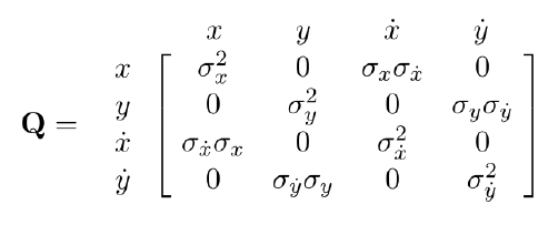
• In practical terms

  \[Q = \begin{bmatrix} \frac{\Delta t^4}{4} & 0 & \frac{\Delta t^3}{2} \\ 0 & \frac{\Delta t^4}{4} & 0 \\ \frac{\Delta t^3}{2} & 0 & \Delta t^2 \\ 0 & \frac{\Delta t^3}{2} & 0 \end{bmatrix} \sigma^2_a\]

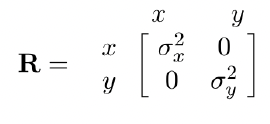
Simple example: tracking a bouncing ball

• Dynamics of a ball is governed by gravity

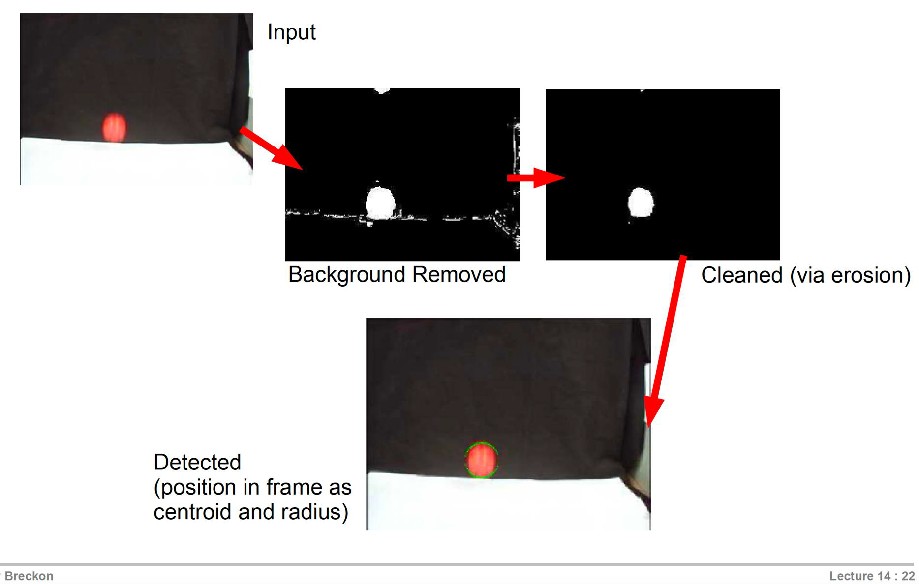
• Say we have an image sequence, captured by a fixed camera

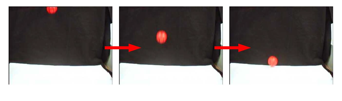
• First of all, we must detect the ball
  • In this case, it is very simple using background modelling
• Then we can use the Kalman filter to track it

The state vector

• Once more, we use the position and velocity information of the ball
  • $s^t = (x^t, y^t, v_x^t, v_y^t)$
• There is some additional information: we can use gravity $g$

  • This will add an acceleration

  • \[a^t = (0, g)\]

Prediction step

• The equation is the usual one, where we can use $\Delta t = 1$

  \[y_t = A x_{t-1} + B \bar u_t\] \[A = \begin{bmatrix} 1 & 0 & \Delta t & 0 \\ 0 & 1 & 0 & \Delta t \\ 0 & 0 & 1 & 0 \\ 0 & 0 & 0 & 1 \end{bmatrix} ,\ B \bar{u}_t = \begin{bmatrix} 0 \\ 0 \\ 0 \\ g \Delta t \end{bmatrix}\]

• Where the matrix $A$ updates the state and $B$ is the external control

  • In our case gravity $g$

Measurement and System

• We can then write the observation matrix as

\[H = \begin{bmatrix} 1 & 0 & 0 & 0 \\ 0 & 1 & 0 & 0 \end{bmatrix}\]

• The measurement noise

\[R = \begin{bmatrix} 0.285 & 0.005 \\ 0.005 & 0.046 \end{bmatrix}\]

• While the system noise

\[Q = 0.01 \times I\]

Are we done? Not quite …

• So far, we have used the position and the velocity of the target
• The problem is that a position does not quite represent a complex target
  • Objects, animals and people do not look the same from different views
  • So, a bounding rectangle changes when a complex target moves
  • We must take this into consideration
• We will have to use the changes width and height of the bounding rectangle of the target, as the target moves

The Model

• We need a state vector that includes both width and height of the tracked bounding rectangle

  • I mentioned earlier on, this is essential because a target usually changes its shape, and this also affects the bounding rectangle

  • \[x_{k-1} = [x, y, v_x, v_y, h, w]\]
• We might want to use another state vector instead, that takes into consideration the velocity of the bounding rectangle
  • $x_{k-1} = [x, y, v_x, v_y, h, w, v_h, v_w]$

What if we want to track a face… or more

• Kalman uses measurement and time updating
• The measurement update equations correspond to the equations used to correct the tracker when the face being tracked is detected and its location in the image is definitive
• The time update equations as defined by Kalman are used to predict the present location of the tracked face when it has not been currently detected in the image space

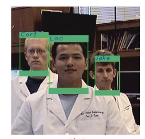
Modelling the state vector

• The Kalman state vector is initialized with five parameters consisting of
  • the x and y coordinates of the upper left bounding point of the face region
  • the velocity in the x and y directions, and
  • the width of the face bounded region
  • The height of the face bounded region is always assumed to be 1.25 times the size of the calculated width

\[\begin{bmatrix} \hat{x}_t \\ \hat{y}_t \\ \dot{x}^t \\ \dot{y}^t \\ W_t \end{bmatrix}\]

Transition matrix

• The x and y coordinates and width of the face region are initially set to the values given by the face detection process
• … while the velocity values of the state vector are set to 1
• The state-space representation of each tracker is given as

\[\begin{bmatrix} \hat{X}_t \\ \hat{Y}_t \\ \hat{X}'_t \\ \hat{Y}'_t \\ \hat{W}_t \end{bmatrix} = \begin{bmatrix} 1 & 0 & \Delta t & 0 & 0 \\ 0 & 1 & 0 & \Delta t & 0 \\ 0 & 0 & 1 & 0 & 0 \\ 0 & 0 & 0 & 1 & 0 \\ 0 & 0 & 0 & 0 & 1 \end{bmatrix} \begin{bmatrix} x_{t-1} \\ y_{t-1} \\ x'_{t-1} \\ y'_{t-1} \\ W_{t-1} \end{bmatrix} + w_t\]

How does Kalman work in this case?

• When a face is occluded or because of a poor pose angle, the tracker predicts the motion
• When faces are detected and matched with a tracker system, they are then given as measurement input to the Kalman filter
• The Kalman tracker then uses this data to effectively correct the system and obtain a probable state vector

\[\left.\left[ \begin{array} {c}x_t \\ y_t \\ x_t \\ y_t^{\prime} \\ W_t \end{array}\right.\right]= \begin{bmatrix} \hat{x}_t \\ \hat{y}_t \\ \hat{x}_t^{\prime} \\ \hat{y}_t^{\prime} \\ \hat{W}_t \end{bmatrix}+K_t\left\{ \begin{bmatrix} mx_t \\ my_t \\ mW_t \end{bmatrix}- \begin{bmatrix} 1 & 0 & \Delta t & 0 & 0 \\ 0 & 1 & 0 & \Delta t & 0 \\ 0 & 0 & 0 & 0 & 1 \end{bmatrix} \begin{bmatrix} \hat{x}_t \\ \hat{y}_t \\ \hat{x}_t^{\prime} \\ \hat{y}_t^{\prime} \\ \hat{W}_t \end{bmatrix}\right\}\]

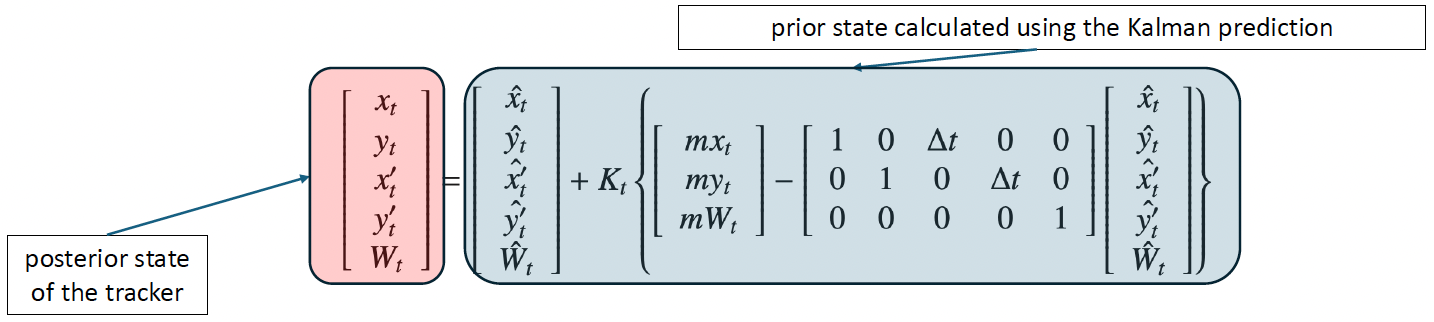
• $K_t$ is the Kalman gain factor which is based on the error of the tracker, and $m x_t, m y_t,$ and $m W_t$ form the measurement vector where the $x, y$ coordinate and width of the input face region is measured.
• These equations allow the tracking system to be properly corrected so that the process remains seamless.

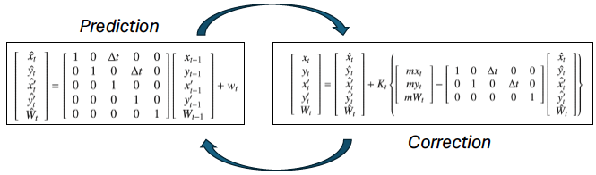
Prediction and Correction

• Using the prediction and correction methods described in equations 1 and 2 as a basis for the tracking unit, the multiple face tracking system defines an independent unit to each distinct person being tracked.

Mean-shift

• The Mean-shift algorithm is an efficient approach to perform segmentation and can also be employed to track objects
• It is a mode seeking algorithm, based on an old method by Fukunaga and Hostetler (1975)
• Mean-shift is used to track non-rigid objects, (a person, for instance)
  • Objects for which it is hard to specify an explicit 2D parametric motion model
• Appearances of non-rigid objects can sometimes be modeled with color distributions

In other words …

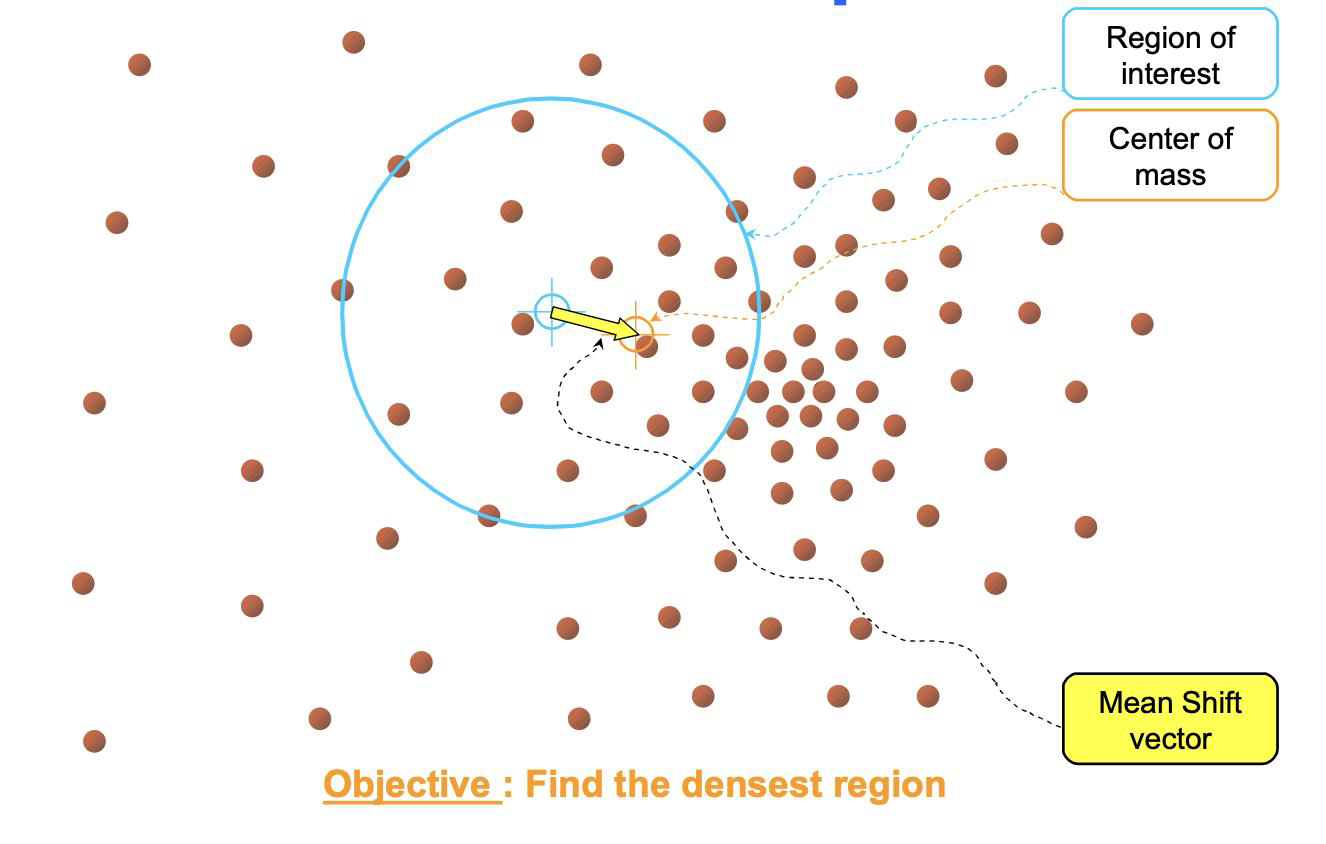
• The mean shift algorithm is a non-parametric clustering technique that identifies clusters in data by iteratively shifting data points towards the denser regions of the data distribution.
• Essentially it implements “climbing uphill” to find the peaks in the density function, without requiring prior knowledge of the number of clusters present.
• It achieves this by calculating the “mean shift” vector, which points in the direction of the maximum density increase within a local window around each data point, and then updating the data point’s position accordingly until convergence is reached.

Mode in statistics

Mode The value that appears most frequently in a data set. A set of data may have one mode, more than one mode, or no mode at all.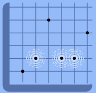

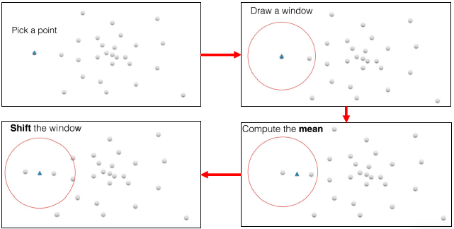
Intuitive description

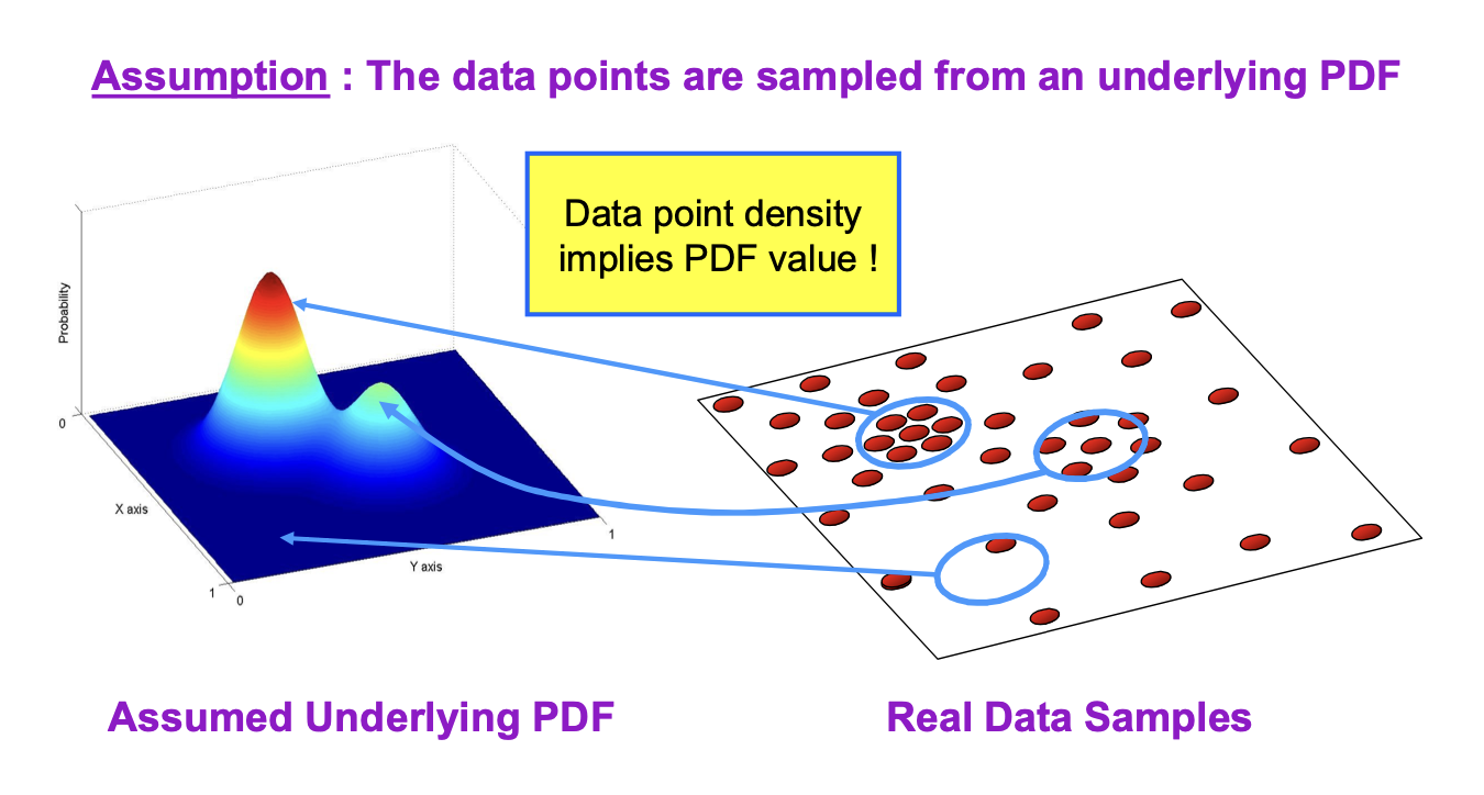
Non-parametric density estimation

We can use a Gaussian kernel

Normal kernel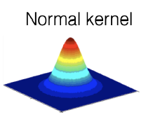

\[K(x, x') = c \exp\left(-\frac{1}{2} \|x - x'\|^2\right)\]

Kernel Density Estimation (KDE)

• In the example I gave you in the last workshop, we have modelled a colour patch with a single Gaussian distribution
• If you took a good look at the distribution of a patch in the $(r, g)$ space, you would have noticed that the distribution is far from being Gaussian
• In general, the data distribution is sometimes too irregular and does not resemble any of the usual PDF
• The Kernel Density Estimator (KDE) provides a rational and visually pleasant representation of the data distribution

How does KDE work?

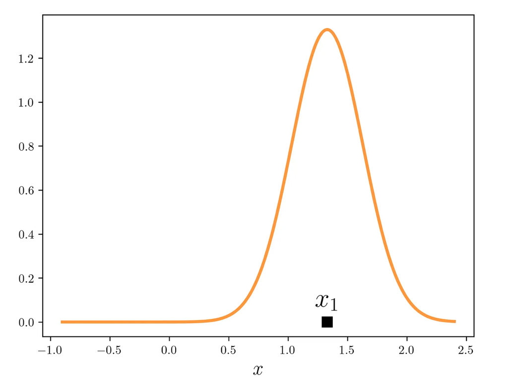
• The KDE method makes use of building blocks
• The distinctive feature of KDE is that it employs only one type of brick, known as the kernel (‘one brick to rule them all’)
• The key property of this brick is the ability to shift and stretch/shrink
• Each datapoint is given a brick, and KDE is the sum of all bricks

The Gaussian function is used

• The building brick we wanted is the Kernel function
• This Kernel is equivalent to a Gaussian distribution with zero mean and unit variance

\[K(x) = \frac{1}{\sqrt{2\pi}} \exp\left[-\frac{x^2}{2}\right]\]

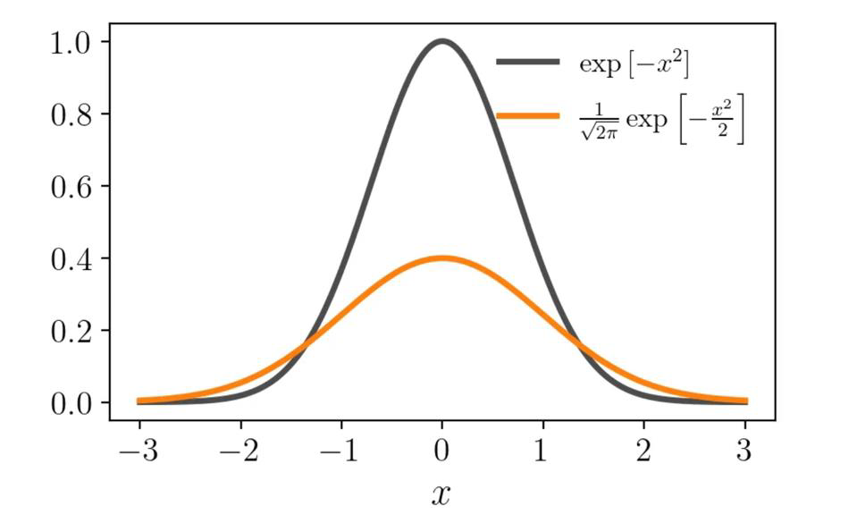
Properties

• The Kernel we chose can be shifted along the axis $K(x - x_i)$

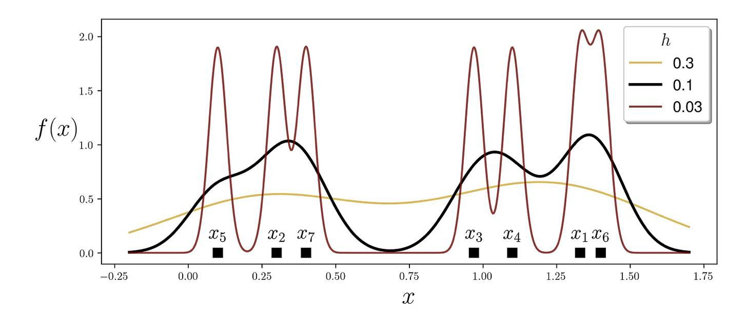
• Its bandwidth can be tuned by dividing the argument by h

  \[\frac{1}{h}K\left(\frac{x - x_i}{h}\right)\]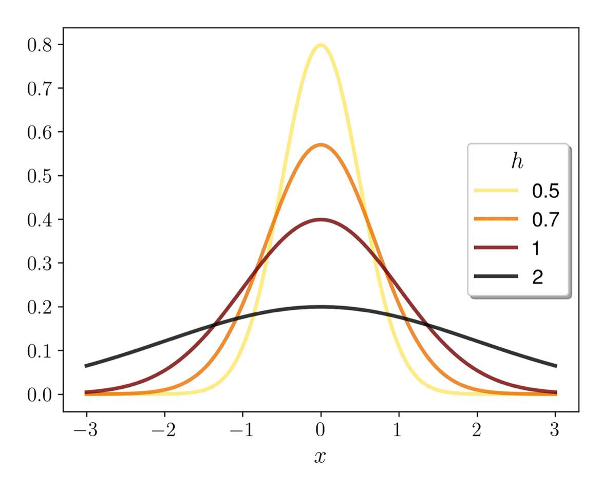
• 

  Example

\[\frac{1}{h}K\left(\frac{x - x_1}{h}\right)\]

# dataset
x = [1.33, 0.3, 0.97, 1.1, 0.1, 1.4, 0.4]

# bandwidth
h = 0.3

\[f(x) = \frac{1}{2h}\sum_{i=1}^{2} K\left(\frac{x - x_i}{h}\right)\]

Full picture

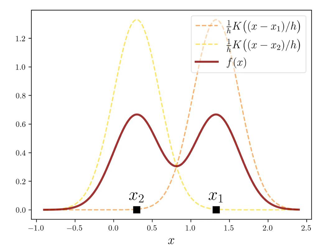
• We use all the data points $X = [x_1, x_2, \ldots, x_n]$

• We end up with the following kernel density estimator

  \[f(x) = \frac{1}{nh} \sum_{i=1}^{n} K\left(\frac{x - x_i}{h}\right)\]

In our example

# dataset
x = [1.33, 0.3, 0.97, 1.1, 0.1, 1.4, 0.4]

# bandwidth
h = 0.3

Implementing it in Python

# v1
import numpy as np
import matplotlib as plt

# the Kernel function
def K(x):
    return np.exp(-x**2/2)/np.sqrt(2*np.pi)

# dummy dataset
dataset = np.array([1.33, 0.3, 0.97, 1.1, 0.1, 1.4, 0.4])

# x-value range for plotting KDEs
x_range = np.linspace(dataset.min()-0.3, dataset.max()+0.3, num=600)

# bandwidth values for experimentation
H = [0.3, 0.1, 0.03]
n_samples = dataset.size

# line properties for different bandwidth values
color_list = ['goldenrod', 'black', 'maroon']
alpha_list = [0.8, 1, 0.8]
width_list = [1.7, 2.5, 1.7]

plt.figure(figsize=(10,4))

# v2
# iterate over bandwidth values
for h, color, alpha, width in zip(H, color_list, alpha_list, width_list):
    total_sum = 0
    # iterate over datapoints
    for i, xi in enumerate(dataset):
        total_sum += K((x_range - xi) / h)
        plt.annotate(r'$x_{}$'.format(i+1),
                     xy=[xi, 0.13],
                     horizontalalignment='center',
                     fontsize=18,
                     )
    y_range = total_sum/(h*n_samples)
    plt.plot(x_range, y_range,
             color=color, alpha=alpha, linewidth=width,
             label=f''
             )
plt.plot(dataset, np.zeros_like(dataset), 's',
         markersize=8, color='black')

plt.xlabel(r'$x$', fontsize=22)
plt.ylabel(r'$f(x)$', fontsize=22, rotation='horizontal', labelpad=20)
plt.legend(fontsize=14, shadow=True, title=r'$h$', title_fontsize=16)
plt.show()

The Mean-shift algorithm

Given a set of points:

\[\{x_s\}_{s=1}^S \quad x_s \in \mathbb{R}^d\]

and a kernel:

\[K(x, x')\] \[K(x, x') = c \exp\left(-\frac{1}{2} \|x - x'\|^2\right)\]

Find the mean sample point:

\[x\]

Initialize $x$

While $v(x) > \epsilon$

1. Compute mean-shift

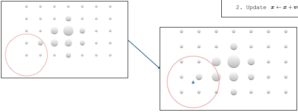
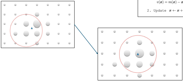
   \[m(x) = \frac{\sum_s K(x, x_s)x_s}{\sum_s K(x, x_s)}\] \[v(x) = m(x) - x\]

2. Update $x \leftarrow x + v(x)$

Mean-shift in images

\[\{x_s\}_{s=1}^S \quad x_s \in \mathbb{R}^d\]

Associated weights:
$w(x_s)$

Sample mean:

\[m(x) = \frac{\sum_s K(x, x_s) w(x_s) x_s}{\sum_s K(x, x_s) w(x_s)}\]

Mean shift:

\[m(x) - x\]

For images, each pixel is point with a weight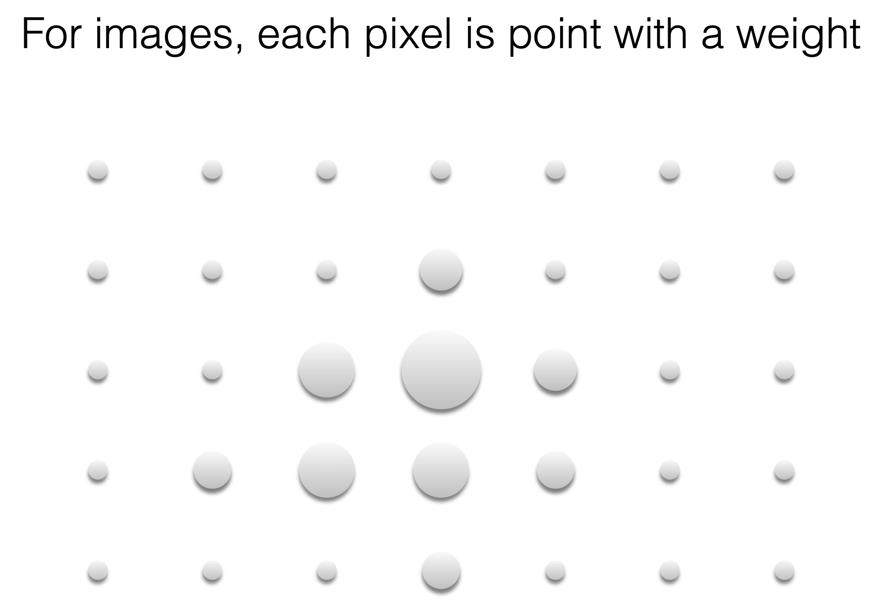

Given a point, find the local mean

Goal: find the best candidate location in frame 2

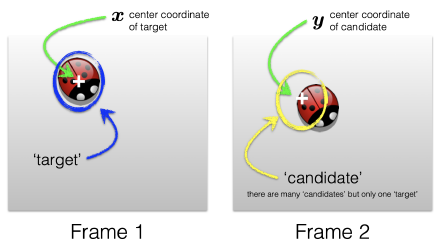
Use the mean shift algorithm to find the best candidate location

Non-rigid object tracking

Search for similar descriptor in neighborhood in next frame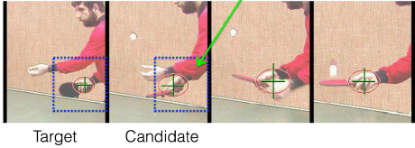

CAMshift and reference

• The CAMshift algorithm was published in 1998
• The problem was to find a solution to track faces in an intelligent user interface
• It is an extension of the Mean-shift, that makes possible the resizing of the window
• Check this Web page for more details
  • https://datahacker.rs/object-tracking-with-mean-shift-and-camshift-algorithms/

Summary

• We have seen the Kalman filter a bit more in detail
• We have studied simple examples
• We have learnt that objects change their shape when captured by a camera
  • This means their bounding boxes should also be included as part of the state vector
• We have learnt about KDE and the Mean-Shift algorithm
  • This is used for image segmentation, but can also be used for tracking a moving target