2025-09-08-Digital and Optimal Control 2 Analysis of discrete-time systems using *z*-transforms

ELEC-E8101: Digital and Optimal Control 2 Analysis of discrete-time systems using z-transforms

In the previous lecture. . .

We

• Discussed the importance of feedback control
• Listed, advantages and disadvantages of digital control
• Discussed the implications of converting continuous-time models into discrete-time models
• Derived and used the properties of Laplace transforms to represent continuous-time systems

Questions and feedback from last week

• Good recap and reminder of what parts of the memory need to be refreshed
• In-class exercise and examples were good
• There could have been some hints after some time in the self study exercise
• A bit slower
• What is the difference between the design principles?

Discrete-time controller design

There are 2 main design approaches

• Discretize the analog controller

• Discretize the process and do the entire design in discrete time

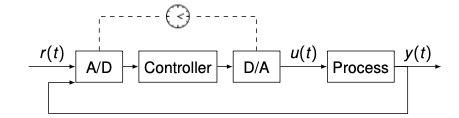
Approach 1

• Discretize the analog controller

• Assume we have a transfer function $G(s)$ given in the Laplace domain that describes our process
• We now design a controller $K(s)$ in the Laplace domain
• Then we discretize this controller so we can implement it on a microcontroller
• This is what we did in the disk drive example last week!

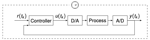
Approach 2

• Discretize the process and do the entire design in discrete time

• Assume again we have a model of the process in the Laplace domain, $G(s)$
• We now discretize the process (how? → next week), i.e., we get a transfer function $H(z)$ in the z-domain (we will discuss the z-domain today)
• Then, we design the controller $K(z)$ directly using the discrete-time transfer function

Learning outcomes

By the end of this lecture, you should be able to:

• Explain the importance of z-transforms for analyzing discrete-time systems
• Derive and use the properties of z-transforms
• Represent discrete-time sequences in z-transform
• Analyze discrete-time systems
• Define the transfer function of a linear time-invariant (LTI) system
• Determine whether or not the transfer function is causal and stable

Recap and introduction

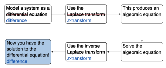
• In the last lecture, we discussed the Laplace transform
• It turns differential equations into algebraic terms with respect to s
• For discrete-time system, we use the z-transform
• z-transform turns difference equations into algebraic terms with respect to z

Introduction

• Analog systems are designed and analyzed with the use of Laplace transforms
• Discrete-time systems are analyzed using a similar technique, called z-transforms

Historical note During and after World War II, a lot of activity was devoted to analysis of radar systems. These systems are naturally sampled because a position measurement is obtained once per antenna revolution. First steps by Hurewicz (1947) – later defined as the z-transform by Ragazzini and Zadeh (1952).

• Basic idea the same for Laplace and z-transforms:
  • After determining the impulse response of the system, the response to any other input signal can be extracted by simple arithmetic operations
  • The behavior and the stability of the system can be predicted from the zeros and poles of the transfer function

Recap: why are we interested in digital control?

• Many application examples use microcontrollers, i.e., work in discrete time: robots, cars, chemical processes, …
• But the underlying dynamics are continuous…
• → We need to discretize them, which we will discuss in the next lecture
• For today, let’s consider a system that naturally evolves in discrete time

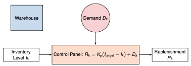
Digital inventory management system

• Consider a system that tracks and controls the inventory of items in a warehouse
• The inventory levels $I_k$ are updated at discrete time intervals $k \to k + 1$ (e.g., daily or weekly), and decisions about replenishments $R_k$ are made at these intervals based on the current inventory level, the target inventory level $I_{\text{target}}$, and demand $D_k$
• We have
  \(I_{k+1} = I_k - D_k + R_k = I_k - D_k + K_p (I_{\text{target}} - I_k) + D_k\)
• How do we need to choose $K_p$ to have $I_k \to I_{\text{target}}$ as $k \to \infty$?

From Laplace transform to z-transform

• The Laplace transform is given by
  \(\mathcal{L}\{x(t)\} := X(s) = \int_{t=-\infty}^{+\infty} x(t) e^{-st} \, dt\)

• s is a complex number and substituting $s = \sigma + j\omega$, we get
  \(X(\sigma, \omega) = \int_{t=-\infty}^{+\infty} x(t) e^{-(\sigma + j \omega) t} \, dt\)

• Step 1: change the signal from continuous time to discrete, i.e., $x(t) \rightarrow x_k$
  \(X(\sigma, \omega) = \sum_{k=-\infty}^{+\infty} x_k e^{-(\sigma + j \omega) k}\)

• Step 2: define $r = e^\sigma$ and $z = r e^{j \omega}$ to obtain the standard form of the z-transform:
  \(\mathcal{Z}(x_k) := X(z) = \sum_{k=-\infty}^{+\infty} x_k z^{-k}\)

Example: discrete-time impulse

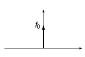
• The sequence ${ f_0, 0, 0, \ldots }$ is an impulse (pulse) with strength $f_0$, i.e.,

\[f_k = f_0 \delta_k\]

where

\[\delta_k = \begin{cases} 1 & \text{if } k = 0 \\ 0 & \text{if } k \neq 0 \end{cases}\]

• Find the $z$-transform of $f_k$

Example: discrete-time impulse – solution

• Write down the definition of the z-transform

\[\mathcal{Z}(f_{k}) = \sum_{k=-\infty}^{\infty} f_{k} z^{-k}\]

• Insert the discrete-time impulse

\[\sum_{k=-\infty}^{\infty} f_{k} z^{-k} = \sum_{k=-\infty}^{\infty} f_{0} \delta_{k} z^{-k} = f_{0} \left( \ldots + \delta_{-2} z^{2} + \delta_{-1} z^{1} + \delta_{0} z^{0} + \delta_{1} z^{-1} + \delta_{2} z^{-2} + \ldots \right)\]

• Insert definition of the impulse

\[f_{0} \left( \ldots + 0 z^{2} + 0 z^{1} + 1 z^{0} + 0 z^{-1} + 0 z^{-2} + \ldots \right) = f_{0}\]

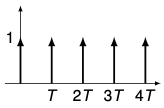
Example: discrete-time (unit) step function

• The sequence ${1, 1, 1, \ldots }$ is a step function with strength 1, i.e.,
  \(u_k = \begin{cases} 1 & \text{if } k \geq 0 \\ 0 & \text{if } k < 0 \end{cases}\)

• The absolute time at instant $k$ is $kT$, where $T$ is the sampling interval
• Find the z-transform of $u_k$

Example: discrete-time (unit) step function – solution

• Start again from the definition of the z-transform and insert the step function

\[\mathcal{Z}(u_k) = \sum_{k=-\infty}^{\infty} u_k z^{-k} = \sum_{k=0}^{\infty} z^{-k} = 1 + z^{-1} + z^{-2} + \ldots\]

→ Geometric series

• General geometric series:

\[\sum_{k=0}^{\infty} a r^k\]

• Converges if $

  r

  < 1$. Then:

\[\sum_{k=0}^{\infty} a r^k = \frac{a}{1-r}\]

• In our case:

\[a = 1, \quad r = z^{-1}\]

→ If $\left

z^{-1} \right

< 1$, we have

\[\mathcal{Z}(u_k) = \frac{1}{1 - z^{-1}} = \frac{z}{z-1}\]

Example: discrete-time exponential function

• Now, we consider the function

\[x_k = a^k u_k, \quad a \in \mathbb{R}\]

where

\[u_k = \begin{cases} 1 & \text{if } k \geq 0 \\ 0 & \text{if } k < 0 \end{cases}\]

• Find the z-transform of $x_k$

Example: discrete-time exponential function – solution

• As before:

\[\mathcal{Z}(x_k) = \sum_{k=-\infty}^{\infty} x_k z^{-k} = \sum_{k=0}^{\infty} a^k z^{-k} = \sum_{k=0}^{\infty} \left( a z^{-1} \right)^k = 1 + a z^{-1} + \left( a z^{-1} \right)^2 + \ldots\]

→ Again geometric series

• Converges if $\left

  a z^{-1} \right

  < 1$. Then

\[\mathcal{Z}(x_k) = \frac{1}{1 - a z^{-1}} = \frac{z}{z - a}\]

• And the region of convergence (ROC) is

\[\text{ROC}_x = \{ z \in \mathbb{C} : |a z^{-1}| < 1 \}\]

More examples

• Consider the function
  \(x_k = -a^k u_{-k-1}, \quad a \in \mathbb{R}\)
  where
  \(u_k = \begin{cases} 1 & \text{if } k \geq 0 \\ 0 & \text{if } k < 0 \end{cases}\)

• Find the z-transform of $x_k$

More examples – solution

• As before
  \(\mathcal{Z}(x_k) = \sum_{k=-\infty}^\infty -a^k u_{-k-1} z^{-k} = -\sum_{k=-\infty}^{-1} (a z^{-1})^k = -\sum_{k=1}^\infty (a^{-1} z)^k = 1 - \sum_{k=0}^\infty (a^{-1} z)^k\)

• Limit exists if $\big| a^{-1} z \big| < 1$. Then,
  \(X(z) = 1 - \frac{1}{1 - a^{-1} z} = \frac{z}{z - a}\)

• And the region of convergence is
  \(\mathrm{ROC}_x = \{ z \in \mathbb{C} : |a^{-1} z| < 1 \}\)

In-class exercise

• Find the z-transform and region of convergence (ROC) of the following difference equation
  \(x_k = a^k u_k - b^k u_{-k-1}, \quad a, b \in \mathbb{R}\)
  where
  \(u_k = \begin{cases} 1 & \text{if } k \geq 0 \\ 0 & \text{if } k < 0 \end{cases}\)

• When is the ROC an empty set?

In-class exercise – solution

• We already found the z-transforms of the two terms in the previous examples
  → We can exploit the linearity of the z-transform (we will prove it in two slides):

\[X(z) = \frac{z}{z - a} + \frac{z}{z - b}\]

• Region of convergence: we need $\left

  az^{-1}\right

  < 1$ and $\left

  b^{-1}z\right

  < 1$

• Thus, we have $

  z

  >

  a

  $ and $

  z

  <

  b

  $

• If $

  a

  >

  b

  $: $\text{ROC}_x = \emptyset$

• If $

  a

  <

  b

  $: $\text{ROC}_x = { z \in \mathbb{C} :

  a

  <

  z

  <

  b

  }$

Right-sided z-transforms

• Right-sided z-transforms are defined as
  \(\mathcal{Z}_{+}(x_k) := \mathcal{Z}(x_k u_k)\)
  where
  \(u_k = \begin{cases} 1 & \text{if } k \geq 0 \\ 0 & \text{if } k < 0 \end{cases}\)

• That is,
  \(\mathcal{Z}_{+}(x_k) := X_{+}(z) = \sum_{k=0}^{+\infty} x_k z^{-k}\)

• We will mostly use right-sided z-transforms from now on

Properties of z-transforms

• Last week, we discussed different properties of Laplace transforms
• For example, linearity, or that the Laplace transform of the time derivative of f(t) is sF(s) − f(0)
• The z-transform has similar properties

Linearity

• Let $x_k$ be the linear combination of $x_k^{(1)}$ and $x_k^{(2)}$ with ROC $\Pi_1$ and $\Pi_2$
• Then:

\[X(z) = \mathcal{Z}(a x_k^{(1)} + b x_k^{(2)}) = \sum_{k=0}^{\infty} (a x_k^{(1)} + b x_k^{(2)}) z^{-k}\] \[= a \sum_{k=0}^{\infty} x_k^{(1)} z^{-k} + b \sum_{k=0}^{\infty} x_k^{(2)} z^{-k} = a X^{(1)}(z) + b X^{(2)}(z)\]

• The ROC is then $\Pi \supseteq \Pi_1 \cap \Pi_2$. Note that $\Pi$ can be bigger

Example

• Consider the function
  \(x_k = a^k u_k - a^k u_{k-1}, \quad a \in \mathbb{R}\)

• These are two exponential functions, thus,
  \(\Pi_1 = \Pi_2 = \{ z \in \mathbb{C} : | a z^{-1} | < 1 \}\)

• For the sum, we have
  \(x(z) = \sum_{k=-\infty}^{\infty} (a^k u_k - a^k u_{k-1}) z^{-k} = \sum_{k=0}^{\infty} (a z^{-1})^k - \sum_{k=1}^{\infty} (a z^{-1})^k = 1\)

• Therefore,
  \(\Pi = \{ z \in \mathbb{C} \supset \Pi_1 \cap \Pi_2 \}\)

Properties of right-sided z-transforms

Delays

\[\mathcal{Z}_+\{x_{k-k_0}\} = z^{-k_0} \left( X_+(z) + \sum_{m=-k_0}^{-1} x_m z^{-m} \right), \quad \text{ROC}_x \text{ except } z=0\]

Proof

\[\begin{aligned} \mathcal{Z}_+\{x_{k-k_0}\} &= \sum_{k=0}^{\infty} x_{k-k_0} z^{-k} \\ &= \sum_{m=-k_0}^{\infty} x_m z^{-(m+k_0)}, \quad m := k - k_0 \\ &= z^{-k_0} \left( \sum_{m=0}^{\infty} x_m z^{-m} + \sum_{m=-k_0}^{-1} x_m z^{-m} \right) \end{aligned}\]

Prediction

\[\mathcal{Z}_{+}\{x_{k+k_0}\} = z^{k_0} \left( X_+(z) - \sum_{m=0}^{k_0-1} x_m z^{-m} \right), \quad \text{ROC}_x \text{ except } z = \infty\]

Proof

\(\begin{aligned} \mathcal{Z}_{+}\{x_{k+k_0}\} &= \sum_{k=0}^\infty x_{k+k_0} z^{-k} \\ &= \sum_{m=k_0}^\infty x_m z^{-(m-k_0)}, \quad m := k + k_0 \\ &= z^{k_0} \sum_{m=k_0}^\infty x_m z^{-m} = z^{k_0} \left( \sum_{m=0}^\infty x_m z^{-m} - \sum_{m=0}^{k_0-1} x_m z^{-m} \right) \end{aligned}\)

Properties of z-transforms

Differentiation in the z-domain

\[\{ x_k \xleftrightarrow[z]{} X(z), \text{ROC}_x \} \implies \left\{ k x_k \xleftrightarrow[z]{} -z \frac{d}{dz} X(z), \text{ROC}_x, \text{ possibly except } z=0 \right\}\]

Proof

\[-z \frac{d}{dz} X(z) = -z \frac{d}{dz} \left( \sum_{k=0}^{\infty} x_k z^{-k} \right)\] \[= z \sum_{k=0}^{\infty} k x_k z^{-k-1}\] \[= \sum_{k=0}^{\infty} k x_k z^{-k} \quad \underbrace{}_{\mathcal{Z} \{ k x_k \}}\]

Initial value theorem (IVT)

\[x_0 = \lim_{z \to \infty} X(z)\]

Proof

\[X(z) = \sum_{k=0}^{\infty} x_k z^{-k} = x_0 \underbrace{z^{-0}}_{=1} + x_1 \underbrace{z^{-1}}_{\to 0 \text{ as } z \to \infty} + \ldots\] \[\lim_{z \to \infty} X(z) = x_0\]

Final value theorem (FVT): for a causal stable (all poles in the unit circle) system, we have

\[x_{\infty} := \lim_{k \to \infty} x_k = \lim_{z \to 1} (z - 1)X(z)\]

Proof
We can write $x_k$ as

\[x_k = (x_0 - x_{-1}) + (x_1 - x_0) + (x_2 - x_1) + \ldots + (x_k - x_{k-1}), \text{ where } x_{-1} = 0\]

Now we take the limit

\[\lim_{k \to \infty} x_k = \lim_{k \to \infty} \lim_{z \to 1} \left( (x_0 - x_{-1})z^0 + (x_1 - x_0)z^{-1} + (x_2 - x_1)z^{-2} + \ldots \right)\] \[= \lim_{z \to 1} \sum_{k=0}^{\infty} (x_k - x_{k-1}) z^{-k} = \lim_{z \to 1} \left( X(z) - X(z-1) \right)\] \[= \lim_{z \to 1} \left( X(z) - z^{-1} X(z) \right)\]

Property	Expression
Linearity	$\mathcal{Z}\left(ax_k^1 + bx_k^2\right) = a \mathcal{Z}\left(x_k^1\right) + b \mathcal{Z}\left(x_k^2\right)$
Delays	$\mathcal{Z}+{x{k-k_0}} = z^{-k_0} \left( X_+(z) + \sum_{m=-k_0}^{-1} x_m z^{-m} \right)$ ROC$_x$ except $z=0$
Predictions	$\mathcal{Z}+{x{k+k_0}} = z^{k_0} \left( X_+(z) - \sum_{m=0}^{k_0-1} x_m z^{-m} \right)$ ROC$_x$ except $z=\infty$
Differentiation	${x_k \xleftrightarrow{\mathcal{Z}} X(z), \text{ROC}_x} \implies \left{ kx_k \xleftrightarrow{\mathcal{Z}} -z \frac{d}{dz} X(z), \text{ROC}_x, \text{ possibly except } z=0 \right}$
Initial value theorem	$x_0 = \lim_{z \to \infty} X(z)$
Final value theorem	$x_\infty := \lim_{k \to \infty} x_k = \lim_{z \to 1} (z - 1) X(z)$

Inverse z-transform

• Implementing the z-transform takes us from the discrete-time domain to the z-domain
• The opposite procedure is the inverse z-transform
• Derivation of the inverse z-transform via the Fourier transform (𝓕)

\[X(z)\big|_{z=re^{j\omega}} = \mathcal{F}\{ x_k r^{-k} \}, \text{ for } r \text{ such that } z \in \text{ROC}\] \[\implies x_k r^{-k} = \mathcal{F}^{-1}\{X(re^{j\omega})\} \text{ (inverse Fourier transform) }\] \[\implies x_k = r^k \frac{1}{2\pi} \int_{\langle 2\pi \rangle} X(re^{j\omega}) e^{j\omega k} d\omega\] \[\implies x_k = \frac{1}{2\pi} \int_{\langle 2\pi \rangle} X(re^{j\omega}) (re^{j\omega})^k d\omega\]

• Now, we want to replace $\omega$ with z
  \(z = re^{j\omega}\) \(\mathrm{d}z = jre^{j\omega} \mathrm{d}\omega = jz \mathrm{d}\omega\) \(\implies \mathrm{d}\omega = \frac{1}{j} z^{-1} \mathrm{d}z\) with $|z| = r$ and $\omega = 0 \dots 2\pi$

• Therefore,
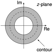
  \(x_k = \mathcal{Z}^{-1}\{X(z)\} = \frac{1}{2 \pi j} \oint X(z) z^{k-1} \mathrm{d}z\)

• Anti-clockwise integration over a closed contour with the ROC of $X(z)$ which includes the intersection of real and imaginary axes of the $z$-complex plane

• Calculation of the integral is quite hard!
• Usually, instead of calculating, we look up the transforms in a table
• These tables only contain some basic functions and cannot cover all cases
• 3 methods for calculating the inverse transform of a function $X(z)$
  • Method of power series expansion
  • Method of partial fraction expansion
  • Method of complex integration (via the residue theorem)

Partial fraction expansion

• Example: find $x_k$ from $X(z)$ given by
  \(X(z) = \frac{1 + 0.5 z^{-1} - 0.32 z^{-2}}{(1 - 0.5 z^{-1})(1 - 0.2 z^{-1})^2}, \quad |z| > 0.5\)

• We perform partial fraction expansion
  \(X(z) = \frac{A}{1 - 0.5 z^{-1}} + \frac{B + C z^{-1}}{(1 - 0.2 z^{-1})^2}\)

• From the 2 equations above, we get
  \(A (1 - 0.2 z^{-1})^2 + (B + C z^{-1})(1 - 0.5 z^{-1}) = 1 + 0.5 z^{-1} - 0.32 z^{-2}\)

• For $z^{-1} = 2$:
  \(0.36 A = 0.72 \implies A = 2\)

• For $z^{-1} = 0$:
  \(A + B = 1 \implies B = 1 - A = 1 - 2 \implies B = -1\)

• For $z^{-1} = 1$:
  \(0.64 A + 0.5 B + 0.5 C = 1.18 \implies C = 2 (1.18 - 1.28 + 0.5) \implies C = 0.8\)

• After doing the partial fraction expansion

\[X(z) = \frac{2}{1 - 0.5 z^{-1}} + \frac{-1 + 0.8 z^{-1}}{(1 - 0.2 z^{-1})^2} = \frac{2}{1 - 0.5 z^{-1}} - \frac{1}{1 - 0.2 z^{-1}} + \frac{0.6 z^{-1}}{(1 - 0.2 z^{-1})^2}\] \[X(z) = \frac{2z}{z - 0.5} - \frac{z}{z - 0.2} + \frac{0.6z}{(z - 0.2)^2}\] \[\implies x_k = 2 (0.5)^k u_k - (0.2)^k u_k + 3k (0.2)^k u_k\]

Power series expansion

• Example: find $x_k$ from $X(z)$ given by

\[X(z) = \frac{1}{1 - az^{-1}}, \quad |z| > |a|\]

• Performing power series expansion

\[\frac{1}{1 - az^{-1}} = 1 + az^{-1} + a^2 z^{-2} + \ldots \quad (\text{converges since } |az^{-1}| < 1)\] \[\implies x_0 = 1, \; x_1 = a, \; x_2 = a^2 \implies x_k = a^k u_k\]

Discrete-time systems

• Example: a first-order difference equation

\[y_{k+1} - ay_k = \delta_k, \quad y_0 = 0\]

and $\delta_k$ is the impulse given by

\[\delta_k = \begin{cases} 1 & \text{if } k = 0 \\ 0 & \text{if } k \neq 0 \end{cases}\]

• Find a solution for $y_k$!

Discrete-time systems – example solution

• Let’s make some calculations directly from the equation:

\[\begin{aligned} y_1 &= ay_0 + \delta_0 &&= 1 \\ y_2 &= ay_1 + \delta_1 &&= a \\ y_3 &= ay_2 + \delta_2 &&= a^2 \\ \vdots \\ y_k &= ay_{k-1} + \delta_{k-1} &&= a^{k-1} \end{aligned}\]

Results: pulse sequence

\[\{a^k\}, k = 0,1,2,\ldots\] \[\mathcal{Z}(y_k) = \sum_{k=1}^{\infty} a^{k-1}z^{-k} = a^{-1} \sum_{k=1}^{\infty} (az^{-1})^{k}\] \[= a^{-1} \frac{az^{-1}}{1 - az^{-1}} = \frac{1}{z - a}, \quad |az^{-1}| < 1\]

• Alternative:

\[zY(z) - z \underbrace{y_0}_{=0} - aY(z) = 1 \quad \Longrightarrow \quad (z - a) Y(z) = 1\] \[\Longrightarrow \quad Y(z) = \frac{1}{z - a} = z^{-1} \frac{z}{z - a} \quad \Longrightarrow \quad y_k = a^{k-1} u_{k-1}\]

Discrete-time systems

• In general, we can describe a discrete-time system as follows

  \[X(z) \xrightarrow{x_k} H(z) \xrightarrow{y_k} Y(z)\]
• $x_k$ represents the input to the system and $y_k$ its output

• Then, we have

  \[Y(z) = H(z)X(z)\]
• $H(z)$ is called the transfer function of the system

• For our previous example

  \[H(z) = \frac{Y(z)}{X(z)} = \frac{1}{z-a}\]
• Initial conditions are ignored

Transfer function of a difference equation

• The difference equation is given by (initial conditions are zero)

\[\sum_{n=0}^{N} a_n y_{k-n} = \sum_{n=0}^{M} b_n x_{k-n}\] \[\Longrightarrow \sum_{n=0}^N a_n z^{-n} Y(z) = \sum_{n=0}^M b_n z^{-n} X(z) \quad \Longrightarrow \quad H(z) = \frac{Y(z)}{X(z)} = \frac{\sum_{n=0}^M b_n z^{-n}}{\sum_{n=0}^N a_n z^{-n}}\]

• We can write it in form of a product

\(H(z) = \frac{b_{\text{M}} \prod_{i=1}^M (z^{-1} - \sigma_i^{-1})}{a_{\text{N}} \prod_{i=1}^N (z^{-1} - \lambda_i^{-1})} = \frac{b'_{\text{M}} \prod_{i=1}^M (z - \tilde{\sigma}_i)}{a'_{\text{N}} \prod_{i=1}^N (z - \tilde{\lambda}_i)}\)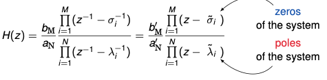

Observations

• Specification of z-transform requires both algebraic expression and ROC
• Rational z-transforms are obtained if the signal is a linear combination of exponentials
  \(Y(z) = \frac{N(z)}{D(z)}\)
• Rational z-transforms are completely characterized by their poles and zeros (except for gain)

Example

• Let’s consider an example transfer function:

\(H(z) = \frac{z}{(z + 0.6)(z - 0.9)}\)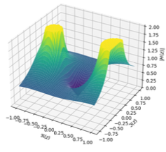

Learning outcomes

By the end of this lecture, you should be able to

• Explain the importance of z-transforms for analyzing discrete-time systems
• Derive and use the properties of z-transforms
• Represent discrete-time sequences in z-transform
• Analyze discrete-time systems
• Define the transfer function of a linear time-invariant (LTI) system
• Determine whether or not the transfer function is causal and stable