2025-09-22-Digital and Optimal Control-Discrete PID controllers

ELEC-E8101: Digital and Optimal Control-Discrete PID controllers

In the previous lecture. . .

We

• Discussed what happens to the signal when sampling
• Derived what is the sampling frequency so that one can reconstruct the signal
• Evaluated the options of discretization in control systems
• Used discretization methods for designing discrete-time systems
• Used direct methods of designing discrete-time systems

Feedback from last week

• Pace still too fast
  → Should definitely get better today

Learning outcomes

By the end of this lecture, you should be able to

• Design practical PID controllers for applications
• Design anti-windup schemes

PID-controllers

• Proportional-integral-derivative (PID) control is the standard for industrial control
• Over 90 % of industrial control systems use PID control
• The ubiquitous nature of PID control stems from
  • Its simple structure
  • The distinct effect of each of the three PID terms
  • Its established use in industry
  • Engineers’ preference to improve existing methods before adopting new ones
• The first theoretical analysis and practical application was in the field of automatic steering systems for ships – early 1920 onward
• Then, used for automatic process control in the manufacturing industry, where it was widely implemented in pneumatic and electronic controllers

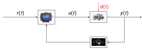
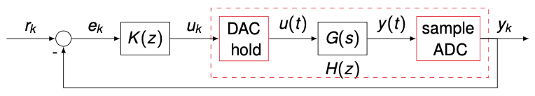
Feedback control in a discrete setting

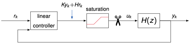
• Let us examine the following block diagram of a control system

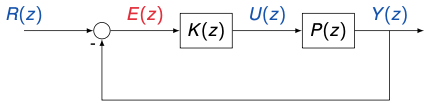
• We have

  \[\begin{aligned} Y(z) &= P(z) U(z) \\ U(z) &= K(z) E(z) \\ E(z) &= R(z) - Y(z) \end{aligned}\]

• Therefore,

  \[Y(z) = P(z) K(z) E(z) = P(z) K(z) ( R(z) - Y(z) )\]

• Solving for $Y(z)$

\[Y(z) = P(z)K(z)E(z) = P(z)K(z)(R(z) - Y(z))\] \[(1 + P(z)K(z))Y(z) = P(z)K(z)R(z) \implies Y(z) = \underbrace{\frac{P(z)K(z)}{1 + P(z)K(z)}}_{:=H(z)} R(z)\] \[\implies H(z) = \frac{Y(z)}{R(z)} = \frac{P(z)K(z)}{1 + P(z)K(z)}\]

• Closed-loop transfer function from reference/input to output

• The block diagram of the control system can be simplified as

\[R(z) \longrightarrow \boxed{H(z) = \frac{P(z)K(z)}{1+P(z)K(z)}} \longrightarrow Y(z)\]

• Similarly, for the error $E(z)$

\[E(z) = R(z) - Y(z) = R(z) - \frac{P(z)K(z)}{1 + P(z)K(z)} R(z)\] \[= \left( 1 - \frac{P(z)K(z)}{1 + P(z)K(z)} \right) R(z) = \frac{1}{1 + P(z)K(z)} R(z)\]

• The problem becomes how to choose an appropriate $K(z)$ such that
  • $H(z)$ will yield desired properties
  • The resulting error function $e_k$ goes to zero as quickly and smoothly as possible

Behavior of continuous 2nd order systems with unit step input

• Consider the following block diagram with a standard 2nd order system

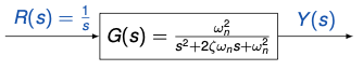
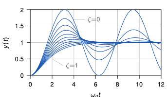
The behavior of the system is fully characterized by

• $\zeta$, the damping factor
• $\omega_n$, the natural frequency

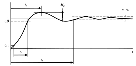
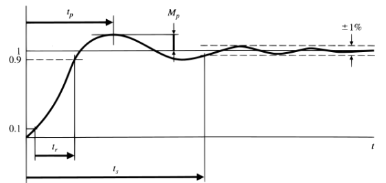
Time domain design specifications

• Typical specifications for the step response (continuous-time) domain

Specification	Expression
Steady-state accuracy	$e_{ss}$
Rise time (10 % – 90 %)	$t_r = \frac{1.8}{\omega_n}$
Peak overshoot	$M_p \approx e^{-\frac{\pi \zeta}{\sqrt{1-\zeta^2}}}$ or $\zeta \geq 0.6 \left( 1 - \frac{M_p \text{ in \%}}{100} \right)$
Settling time (1 %)	$t_s = \frac{4.6}{\zeta \omega_n}$

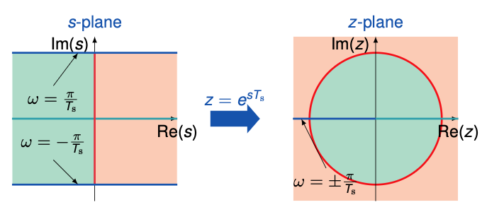
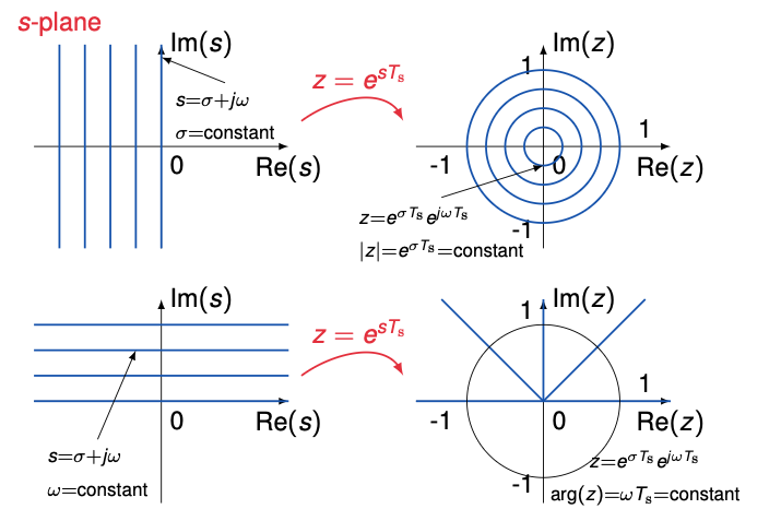
The mapping from the s-plane to the z-plane

• Locus of $s = \sigma + j \omega$ under the mapping $z = e^{sT_s}$

Pole locations for constant damping ratio $\zeta < 1$

\(s^2 + \zeta \omega_0 s + \omega_0^2 = 0\) \(\implies s = -\zeta \pm j \sqrt{1 - \zeta^2} \omega_0\)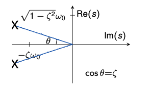

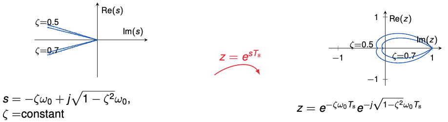
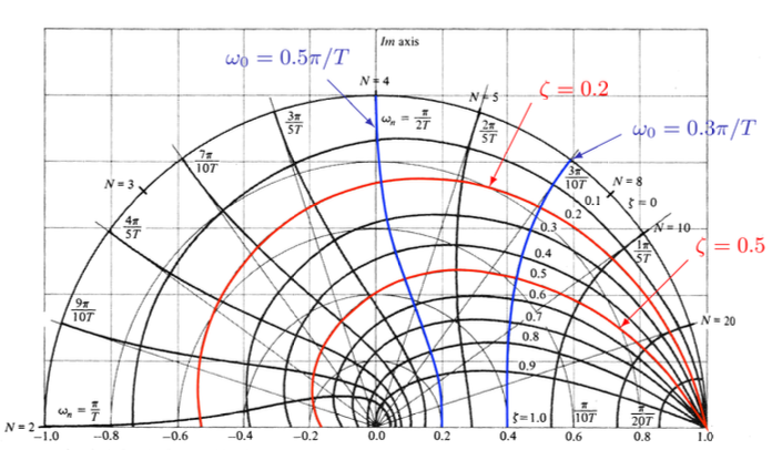
$z = \text{plane loci of roots of constant } \zeta \text{ and } \omega_n$
$s = -\zeta \omega_n \pm j \omega_n \sqrt{1-\zeta^2}$
$z = e^{Ts}$
$T = \text{sampling period}$

Time domain design specifications

• Typical specifications for the step response (discrete-time domain)

Steady-state accuracy
\(e_{ss} = \lim_{z \to 1}(z - 1) E(z)\)

Rise time (10% – 90%)
\(t_r = \frac{1.8}{\omega_n}\)

Peak overshoot
\(M_{\mathrm{p}}\approx e^{-\frac{\pi\zeta}{\sqrt{1-\zeta^{2}}}}\mathrm{or}\zeta\geq0.6\left(1-\frac{M_{\mathrm{p}}\mathrm{in}\%}{100}\right)\)

Settling time (1%)
radius of poles:
\(|z| < 0.01^{\frac{t_s}{t_s}}\)

Example – the car from the last lecture

• We take the transfer function obtained with the Tustin method and set $m = 1 \, t$, $T_s = 10 \, \mathrm{ms}$, and $\beta = 0.01 \, 1/s$:

\[H(z) = \frac{z + 1}{m \left(\left(\frac{1}{T_s} + \beta\right) z + \beta - \frac{2}{T_s}\right)} = \frac{z + 1}{200.01z - 199.99}\]

• Assume the system is controlled by

\[u_k = K_p v_k = 10 v_k\]

• Find the steady-state error to a unit step $e_{ss}$
• Is the step response settling time $t_s < 1$?

Example – steady-state error

• We already showed that
  \(E(z) = \frac{1}{1 + H(z)K(z)} R(z)\)
• Where the input is
  \(R(z) = \frac{z}{z - 1}\)
• And the controller
  \(K(z) = K_p = 10\)
• How do we find the steady-state error?
• What happens for eₖ in the limit?

\[\lim_{k \to \infty} e_k = \lim_{z \to 1} (z - 1) E(z)\] \[= \lim_{z \to 1} (z - 1) \frac{z}{z - 1} \frac{1}{1 + 10 \frac{z+1}{200.01z - 199.99}}\] \[= \lim_{z \to 1} \frac{z(200.01z - 199.99)}{200.01z - 199.99 + 10z + 10}\] \[= \frac{0.02}{20.02} = 0.00099\]

→ We can very precisely track the step input!

Example — settling time

• For the settling time, we said
  \(|z| < 0.01^{\frac{T_s}{t_s}}\)

→ We first need to find the poles of the closed loop system!

\[H_\text{cl}(z) = \frac{H(z)K(z)}{1 + H(z)K(z)} = \frac{10 \frac{z+1}{200.01z - 199.99}}{1 + 10 \frac{z+1}{200.01z - 199.99}} = \frac{10(z+1)}{200.01z - 199.99 + 10(z+1)} = \frac{10(z+1)}{210.01z - 189.99}\]

• Poles are the zeros of the denominator:

\[210.01z - 189.99 \stackrel{!}{=} 0 \implies z = \frac{189.99}{210.01} \approx 0.9\]

→ Then, we check the settling time:

\[0.9 < 0.01^{\frac{0.01}{1}} \implies 0.9 < 0.95 \quad \checkmark\]

Continuous-time PID-controllers

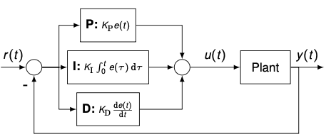
• P: amplifies the error by $K_P$
• I: eliminates the residual error by integrating over its historic cumulative value
• D: looks ahead by exerting control based on the rate of change
• The continuous-time PID-controller in the time domain is

\[u(t) = K_P e(t) + K_I \int_{0}^{t} e(\tau) \, d\tau + K_D \frac{d e(t)}{dt}\]

• And in the Laplace domain:

\(U(s) = \left( K_P + \frac{K_I}{s} + K_D s \right) E(s)\)

P-controller

• The “obvious” method – proportional control

• Example: transfer function $G(s) = \frac{1}{s^2 + s + 1}$ with step input
  

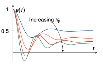
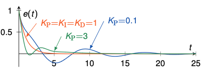
• Higher $K_P$ brings the error $e(t)$ closer to zero but never reaches it
• Also, the overshoot increases

I-controller

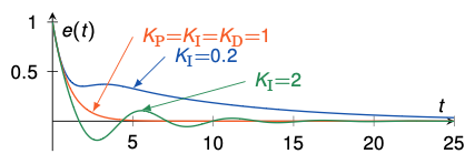
• An integral term increases the action depending on the value of the error and how long it has persisted
• If control action is too small and a steady-state offset remains, the action will increase
• A pure integral controller could bring the error to zero, however
  • It would react slowly in the beginning
  • Once the error is zero, the integral is still non-zero and causes overshoot and oscillations
• Alternative: PI-control, often used for example in motor control

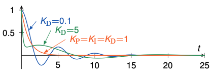
D-controller

• React to changes in the error
  → If error starts to shrink, can decrease control action, otherwise increase
• Aims at flattening error trajectory
• Ideal derivative control cannot (and must not) be realized in a PID-controller
• Practical systems always contain high frequency disturbances, which are amplified by derivative control
• Because of that, a low-pass filter/lag term is usually added

\(K_D s \rightarrow \frac{K_D s}{1 + \frac{K_D s}{N}}\)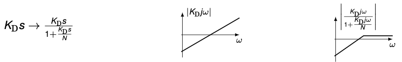

• Other practical modification: take derivative only of the output, not the reference and error signal

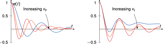
PID-controller

• effect of $K_P$ ($K_I$ and $K_D$ kept constant)

• effect of $K_I$ ($K_P$ and $K_D$ kept constant)

• effect of $K_D$ ($K_P$ and $K_I$ kept constant)

From continuous- to discrete-time PID-controllers

• Simple discretization

\[\left\{ \begin{aligned} P(t) &= K_P e(t) \\ I(t) &= K_I \int_{-\infty}^{t} e(\tau) \, d\tau \\ D(t) &= K_D \frac{d e(t)}{dt} \end{aligned} \right. \implies \left\{ \begin{aligned} P(kT_s) &= K_P e(kT_s) \\ I(kT_s) &= K_I \sum_{n=-\infty}^{k-1} e(nT_s) T_s = K_I T_s \sum_{n=-\infty}^{k-1} e(nT_s) \\ D(kT_s) &= K_D \frac{e(kT_s) - e(kT_s - T_s)}{T_s} = \frac{K_D}{T_s} \Delta e(kT_s) \end{aligned} \right.\]

• Therefore

\[u(kT_s) = K_P e(kT_s) + K_I T_s \sum_{n=-\infty}^{k-1} e(nT_s) + \frac{K_D}{T_s} \Delta e(kT_s)\]

• Taking the z-transform:

\[U(z) = \left( K_P + \frac{K_I T_s}{z - 1} + \frac{K_D}{T_s} \frac{z - 1}{z} \right) E(z)\]

• Note: there are other interpretations of discrete-time PID-controllers
• For example, if backward integration is used in the integral part:

\[H_{\text{PID}}(z) = G_{\text{PID}}(s)\bigg|_{s=\frac{z-1}{zT_s}} = K_{\text{P}} + \frac{K_{\text{I}} T_s z}{z - 1} + \frac{K_{\text{D}}}{T_s} \frac{z - 1}{z}\]

• The discretization of a practical PID-controller is as straightforward

\[\left\{ \begin{aligned} P_m(s) &= K_{\text{P}}(Y_{\text{ref}}(s) - Y(s)) \\ I(s) &= \frac{K_{\text{I}}}{s}(Y_{\text{ref}}(s) - Y(s)) \\ D_m(s) &= - \frac{K_{\text{D}} s}{1 + \frac{K_{\text{D}} s}{N}} Y(s) \end{aligned} \right\} \implies \left\{ \begin{aligned} P_m(z) &= K_{\text{P}}(Y_{\text{ref}}(z) - Y(z)) \\ I(z) &= \frac{K_{\text{I}} T_s}{z-1} (Y_{\text{ref}}(z) - Y(z)) \\ D_m(z) &= D_m(s) \bigg|_{s=\frac{z-1}{zT_s}} = - \frac{\frac{K_{\text{D}} (z-1)}{zT_s}}{1 + \frac{K_{\text{D}}}{N} \frac{z - 1}{zT_s}} Y(z) \end{aligned} \right.\]

Tuning PID-controllers

• The structure of the used discrete PID algorithm must always be told together with the tuning parameters $K_P$, $K_I$, $K_D$ (and $T_s$)
• Controller design is typically based on heuristic design methods for selecting the controller parameters
• The principal design goal is stability: the system is stable when the closed-loop poles are on the left half of the $s$-plane or inside the unit circle in the $z$-plane
• Secondary criteria are, for example, rise time, overshoot, settling time, and steady-state error
• These can be analyzed graphically from impulse, step, and ramp responses of the closed-loop system

Table: Effect of increasing a parameter independently

Parameter	Rise time	Overshoot	Settling time	Steady-state error	Stability
$K_P$	Decrease	Increase	Small change	Decrease	Degrade
$K_I$	Decrease	Increase	Increase	Eliminate	Degrade
$K_D$	Minor change	Decrease	Decrease	No effect in theory	Improve if small

Empirical tuning rules

1. Start with $K_P = K_I = K_D = 0$
2. Increase $K_P$ until you reach the reference value fast with some overshoot and oscillations
3. Increase $K_D$ until the oscillations decrease to a satisfactory level
4. Increase $K_I$ so that steady-state error will be eliminated

Tuning rules for PID controllers
J. G. Ziegler and N. B. Nichols. “Optimum settings for automatic controllers”. In: Transactions of the American Society of Mechanical Engineers 64.8 (1942), pp. 759–765

Actuator saturation

• Most control systems are designed based on linear theory
• A linear controller is simple to implement and performance is good, as long as dynamics remain close to linear
• In practice, we always have nonlinear effects, e.g., actuator saturation, that we need to take care of
• Saturation, if ignored in the design phase, can lead to closed-loop instability, especially if the open-loop process is unstable
• Main reason: the control loop gets broken if saturation is not taken into account by the controller

Saturation function

• Saturation can be defined as the static nonlinearity

\[\text{sat}(u) = \begin{cases} u_{\min}, & \text{if } u < u_{\min}, \\ u, & \text{if } u_{\min} < u < u_{\max}, \\ u_{\max}, & \text{if } u > u_{\max} \end{cases}\]

• $u_{\min}$ and $u_{\max}$ are the minimum and maximum allowed actuation signals
• Example: for a typical DC motor, we have $u_{\min} = -12\,\text{V}, \, u_{\max} = 12\,\text{V}$
• If $u$ is a vector of $m$ components, the saturation function is defined as the saturation of all its components

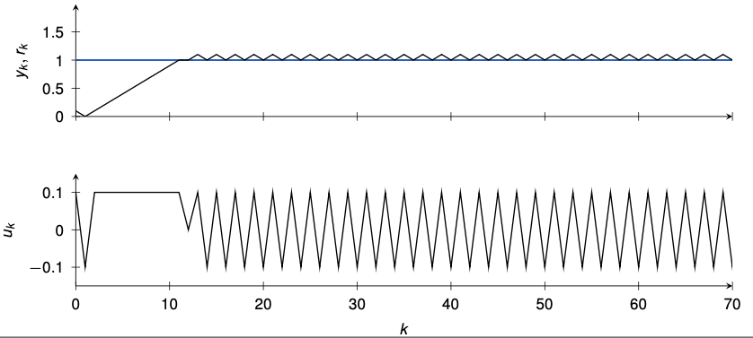
The wind-up problem

• Consider a simple process with saturation (±0.1) and PID gains $K_P = K_I = K_D = 1$

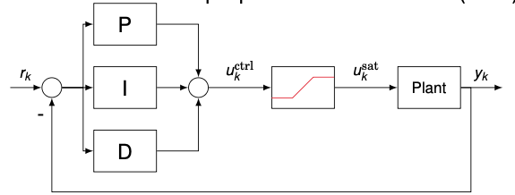
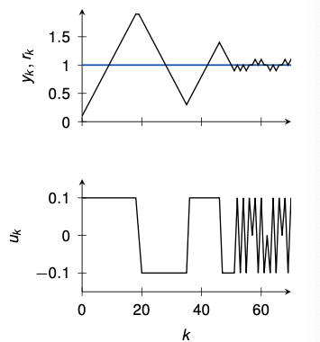
• Slow convergence to steady-state
• The reason is the “wind-up” of the integrator contained in the PID-controller
• The integrator keeps integrating the tracking error even when the input is saturated
• Anti wind-up schemes avoid this effect

Anti-windup #1: incremental algorithm

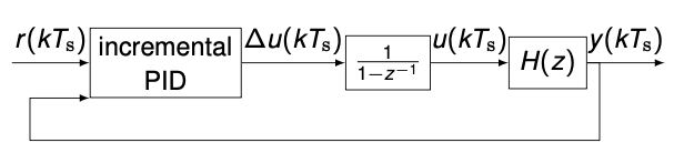
• It only applies to PID control laws implemented in incremental form

\[u((k+1)T_s) = u(kT_s) + \Delta u(kT_s),\]

where

\[\Delta u(kT_s) = u(kT_s) - u((k-1)T_s)\]

• Stop integration if adding a new $\Delta u(kT_s)$ causes a violation of the saturation bound

Anti-windup #2: back-calculation

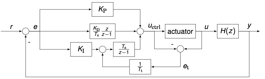
• Anti wind-up scheme has no effect when the actuator is not saturating ( $e_t = 0$ )
• Time constant $T_t$ determines how quickly the integrator of the PID-controller is reset
• If the actual input $u$ of the actuator is not measurable, we can use a mathematical model of it, e.g., $e_t = u_{ctrl} - \text{sat}(u)$

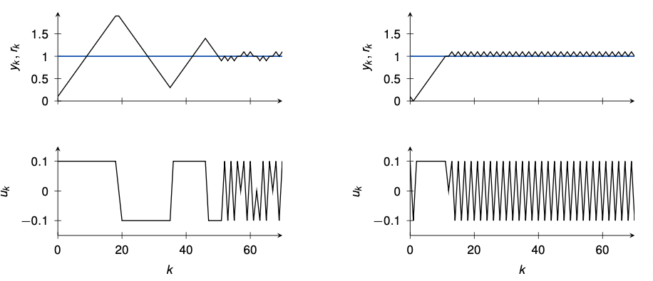
Anti-windup #2: example

• Let’s consider again the PID-controller from before ($K_P = K_I = K_D = 1$) and add back-calculation with $T_t = 1$
• Windup is avoided due to back-calculation
• Note: only one tuning parameter ($T_t$), but only applicable to PID-controllers

Benefits of the anti-windup scheme

• In case of windup we have
  • Large output oscillations
  • Longer time to reach steady-state
  • Peaks of control signal

Hardware demo

Practical demonstration of PID-control: https://youtu.be/fusr9eTceEo

Learning outcomes

By the end of this lecture, you should be able to

• Design practical PID controllers for applications
• Design anti-windup schemes