2025-09-21-Digital and Optimal Control Discretization

Digital and Optimal Control: Discretization

In the previous lecture. . .

We

• Discussed the importance of z-transforms for analyzing discrete-time systems
• Derived and used the properties of z-transforms
• Represented discrete-time sequences in z-transform
• Analyzed discrete-time systems
• Defined the transfer function of a linear time-invariant (LTI) system
• Determined whether or not the transfer function is causal and stable

Feedback and questions from last week

• Pace could be slower
  → I will work on this
• Missing real-life application
  → This will follow today
• “Put a clear legend of each term of the equations”
  → I’m not entirely sure what is meant by a “legend,” but if I get an explanation for that I can try to do this

Where we left last time…

• Let’s consider an example transfer function:

\(H(z) = \frac{z}{(z + 0.6)(z - 0.9)}\)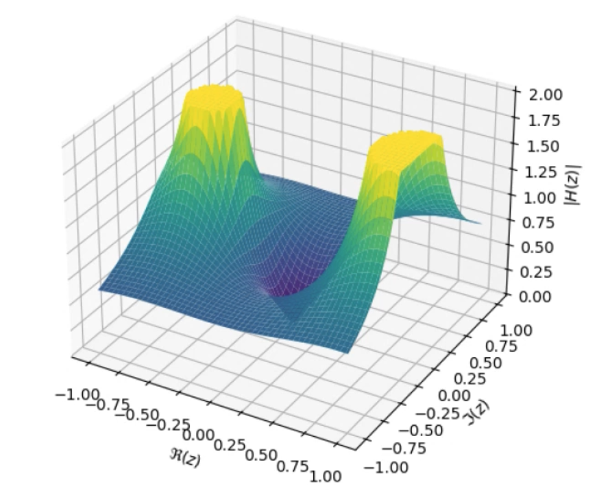

Causal systems

Causal systems We call a system causal if its output $y_{k’}$ only depends on the input $u_k$ for $k \leq k’$.

• Causality in this sense means the future cannot influence the past
• Assume we investigate a system for which $x_k = 0$, for all $k < 0$
• If $h_k$ is causal, then $h_k = 0$, for all $k < 0$, and

\(H(z) = \mathcal{Z}(h_k) = \mathcal{Z}(h_k u_k) = \mathcal{Z}_+(h_k) = H_+(z)\) \(X(z) = \mathcal{Z}(x_k) = \mathcal{Z}(x_k u_k) = \mathcal{Z}_+(x_k) = \mathbf{X_+}(z)\) \(Y(z) = Y_+(z) = \mathcal{Z}(h_k u_k * x_k u_k) = H_+(z) X_+(z)\)

• Details on how this can be derived follow on the next slide. Important conclusion

Conclusion If the transfer function is causal and $x_k = 0, \forall k < 0$, then $\mathcal{Z}_+(\cdot)$ is enough for the analysis of the system.

\(y_k = h_k * x_k = h_k u_k * x_k u_k\) \(= \sum_{n=-\infty}^{\infty} h_n u_n x_{k-n} u_{k-n}\) \(= \sum_{n=0}^{\infty} h_n x_{k-n} u_{k-n}\) \(\Longrightarrow y_k = \sum_{n=0}^k h_n x_{k-n} \Longrightarrow y_k = 0, \forall k < 0\) \(\Longrightarrow Y(z) = Y_+(z) = \mathcal{Z}(h_n u_n * x_n u_n) = H_+(z) X_+(z)\)

• Suppose the transfer function is causal, i.e., $h_k = 0, \forall k < 0$

\[\implies \text{ROC}_h = \{ z \in \mathbb{C} : |z| > \max_{i=1,...,N} |\lambda_i| \}\]

\(H(z) = \sum_{k=0}^{\infty} h_k z^{-k} \implies \text{ROC}_h \text{ includes } z = \infty\)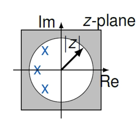

• Suppose

\[\sum_{n=0}^N a_n y_{k-n} = \sum_{n=0}^M b_n x_{k-n} \implies H(z) = \frac{b_0 + b_1 z^{-1} + \dots + b_M z^{-M}}{a_0 + a_1 z^{-1} + \dots + a_N z^{-N}}\]

• Then, the $\text{ROC}_h$ is right-sided and its radius is higher than the maximum pole

Conclusion 1 A discrete-time system $h$ is causal if, and only if, the $\text{ROC}_h$ is the external area of a circle and includes infinity.

Relation between causality and stability

• Suppose the system is stable. Then, $|h|1 := \sum{k=0}^{\infty}

  h_k

  < \infty$

• Consequently, $H(e^{j\omega}) = \mathcal{F}(h_k)$ exists. Therefore, $\text{ROC}_h$ should include $

  z

  =1$

Conclusion 2
A discrete-time system $h$ is bounded-input bounded-output (BIBO) stable if, and only if, $\text{ROC}_h$ includes $z = 1$.

• Combine Conclusions 1 and 2

Theorem
A causal linear time-invariant (LTI) system $h$ with rational $H(z)$ is stable if, and only if, all the poles $\lambda_i$ of $H(z)$ satisfy
\(|\lambda_i| < 1.\)

z-transform: valuable tool

• Efficient calculation for the response of an LTI system: The convolution in the discrete-time domain is computed as a product in the z-domain:
  \(y_k = x_k * h_k \implies Y(z) = X(z)H(z)\)

• Description of LTI systems with regard to their behavior in the frequency domain:
  low pass filter, band pass filter, etc.

• Stability analysis of an LTI system:
  (via calculation of the region of convergence)

  • A causal continuous-time system is stable if its poles are in the left s-half-plane
  • A causal discrete-time system is stable if its poles are located inside the unit circle

Back to the inventory management example

• How can we use the z-transform to analyze the inventory level?
• The dynamics of the process are

\[I_{k+1} = I_k - D_k + R_k\]

• Let’s analyze for which $K_p$ in the control law below the system is stable, i.e., $I_k - I_{\text{target}}$ goes to zero for $k \to \infty$!

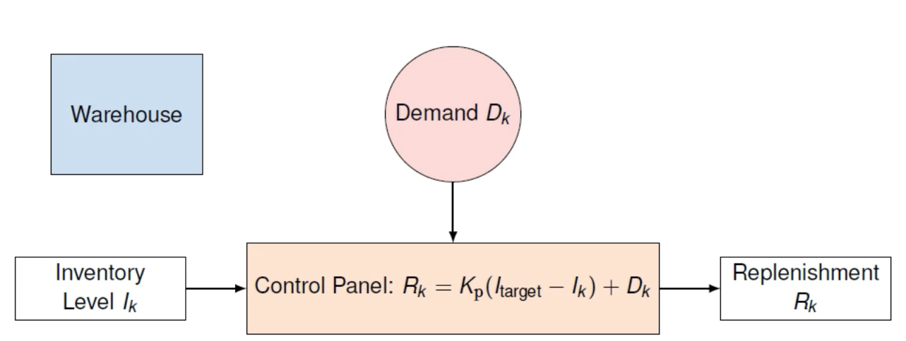
Digital inventory management system

• We have
  \(I_{k+1} = I_k - D_k + R_k\) \(R_k = K_p (I_{\text{target}} - I_k) + D_k\)

• Let’s write this into one equation
  \(I_{k+1} = I_k - D_k + K_p (I_{\text{target}} - I_k) + D_k\) \(= I_k + K_p (I_{\text{target}} - I_k)\)

• We can now use the z-transform
  \(z I(z) = I(z) + K_p (I_{\text{target}} - I(z))\)

• Now we can compute the transfer function
  \(I(z)(z - 1 + K_p) = K_p I_{\text{target}}\) \(\frac{I(z)}{I_{\text{target}}} = \frac{K_p}{z - 1 + K_p}\)

→ The system is stable if $0 < K_p < 2$

Learning outcomes

By the end of this lecture, you should be able to:

• Explain what happens to the signal when sampling
• Derive what is the sampling frequency so that one can reconstruct the signal
• Evaluate different options for discretizing a control system
• Use discretization methods for designing discrete-time systems
• Use direct methods of designing discrete-time systems

Sampling: the bridge from continuous to discrete

• The world surrounding us is analog!
• Signal analysis and control is done via digital computers (see first lecture)
• Thus, analog signals and systems have to be transformed to discrete and vice-versa
• This is done via sampling
• The measured entities are called samples
• The sampling typically takes place in regular intervals, e.g., every $T_s$:

\[x_k := x(kT_s)\]

sssss ……

\[x_p(t) = x_c(t)p(t) = \sum_{n=-\infty}^{\infty} x_c(t)\delta(t - nT_s) = \sum_{n=-\infty}^{\infty} x_c(nT_s)\delta(t - nT_s)\]

where

\[\delta(t - nT_s) = \begin{cases} 1, & \text{if } t = nT_s \\ 0, & \text{otherwise} \end{cases}\]

Frequency range

• Suppose that the Fourier transform of $x_p(t)$ exists, i.e., \(\mathcal{F}\{x_p(t)\} = X_p(j\omega)\)
• Then, \(X_p(j\omega) = \mathcal{F}\{x_p(t)\} = \mathcal{F}\{x_c(t)p(t)\} = \frac{1}{2\pi} X_c(j\omega) * P(j\omega)\)

• Since $p(t)$ is periodic \(p(t) = \sum_{k=-\infty}^\infty a_k e^{j k \omega_s t} \qquad \text{Fourier series}\)

  \[a_n = \frac{1}{T_s} \int_{-\frac{T_s}{2}}^{\frac{T_s}{2}} p(t) e^{-j n \omega_s t} dt = \frac{1}{T_s} \int_{-\frac{T_s}{2}}^{\frac{T_s}{2}} \delta(t) e^{-j n \omega_s t} dt = \frac{1}{T_s}, \ \forall n\] \[\implies p(t) = \frac{1}{T_s} \sum_{k=-\infty}^\infty e^{j k \omega_s t}\]

• Moreover, \(\mathcal{F}\{ e^{j k \omega_s t} \} = 2\pi \delta(\omega - k \omega_s) \implies P(j \omega) = \frac{2\pi}{T_s} \sum_{n=-\infty}^\infty \delta(\omega - n \omega_s), \quad \omega_s = \frac{2\pi}{T_s}\)

• As a result:

\[X_p(j\omega) = \frac{1}{T_s} \sum_{n=-\infty}^\infty X_c(j\omega) * \delta(\omega - n \omega_s)\] \[= \frac{1}{T_s} \sum_{n=-\infty}^\infty X_c(j(\omega - n \omega_s)) * \delta(\omega) \quad (\text{property of convolution})\] \[\Longrightarrow X_p(j\omega) = \frac{1}{T_s} \sum_{n=-\infty}^\infty X_c(j(\omega - n \omega_s))\]

• As a result:

\[X_p(j\omega) = \frac{1}{T_s} \sum_{n=-\infty}^{\infty} X_c(j\omega) * \delta(\omega - n\omega_s)\] \[= \frac{1}{T_s} \sum_{n=-\infty}^{\infty} X_c(j(\omega - n\omega_s)) * \delta(\omega) \quad \text{(property of convolution)}\] \[\implies X_p(j\omega) = \frac{1}{T_s} \sum_{n=-\infty}^{\infty} X_c(j(\omega - n\omega_s))\]

sss

ssss

Sampling criterion/theorem

• Suppose $x_c(t)$ is a low-pass signal with $X_c(j\omega) = 0, \forall

  \omega

  > \omega_0$, e.g.,

• Then, $x_c(t)$ can be uniquely determined by its samples $x_c(nT_s), n=0, \pm 1, \pm 2, \ldots$, if the sampling angular frequency is at least twice as big as $\omega_0$, i.e.,

  \[\omega_s = \frac{2\pi}{T_s} > 2 \omega_0\]
• The minimum sampling angular frequency for which the inequality holds is called the Nyquist angular frequency.

Remarks

• Reconstructing such a signal requires a low-pass filter with cut-off frequency:
  \(\omega_0 < \omega_c < \omega_s - \omega_0\)

• From the natural meaning of frequency, we understand that the fast changes of a signal in time domain correspond to the existence of high frequencies with energy

• The bigger the bandwidth of a signal, the faster the changes in time domain

• Signals with a limited bandwidth are called band-limited
• If a signal is not band-limited, then its perfect reconstruction is impossible
• We should choose the sampling frequency $\omega_s$ to be
  • high enough, so that information loss is small
  • small enough, so that the system does not run out of memory
  • Engineering rule of thumb: we often choose the sampling frequency such that $\omega_s \approx 10\omega_0$
• The reconstruction of a signal might be adequate if $X(j\omega)$ reduces to zero fast for $\omega \to \infty$, which is the case in most practical systems

Sampling with zero-order hold (ZOH)

• Sampling narrow and large-amplitude pulses which approximate impulses are in practice difficult to generate and transmit
• Therefore, it is often more convenient to generate the sampled signal in a form referred to as zero-order hold (ZOH)
• Such a system samples $x_c(t)$ at a given instant and holds that value until the next instant

\[x_0(t) = x_P(t) * g_0(t)\] \[= \sum_{n=-\infty}^\infty x_c(nT_s) \delta (t - nT_s) * g_0(t)\] \[= \sum_{n=-\infty}^\infty x_c(nT_s) \delta (t) * g_0(t - nT_s)\] \[\implies x_0(t) = \sum_{n=-\infty}^\infty x(nT_s) g_0(t - nT_s)\]

Discretization

• There are 2 main design approaches
  (a) Discretize the analog controller

  (b) Discretize the process and do the design completely in discrete time

Discretization methods

• We will see how we can transform the transfer function $G(s)$ of an analog system in the $s$-domain to an equivalent transfer function $H(z)$ of a discrete system in the $z$-domain
• $G(s)$ can be transformed to $H(z)$ by 3 different approaches:
  1. Rely on the use of numerical methods for solving differential equations describing the given system and for converting them to difference equations
  2. Match the response of continuous-time systems to specific inputs (e.g., impulse, step, and ramp functions) to those of discrete-time systems for the same inputs
  3. Match the poles and zeros of $G(s)$ in the $s$-domain with the corresponding poles and zeros of $H(z)$ in the $z$-domain

	s-domain	z-domain
pole	$s = s_0$	$z = e^{s_0 T_s}$

Backward difference method

• Calculate the derivative by using the difference between the current and the previous sample divided by the sampling period, i.e.,
  \(\frac{\mathrm{d}}{\mathrm{d}t}y(t)\big|_{t=kT_s} \approx \frac{y(kT_s)-y([k-1]T_s)}{T_s} = \frac{y_k - y_{k-1}}{T_s}\)

• The Laplace-transform of the derivative is $\mathcal{L}(\dot{y}(t))=sY(s)$
• The $z$-transform of its approximation is
  \(\mathcal{Z}\left(\frac{\mathrm{d}}{\mathrm{d}t} y(t)\big|_{t=kT_s}\right) = \mathcal{Z}\left(\frac{y_k - y_{k-1}}{T_s}\right) = \frac{1-z^{-1}}{T_s}Y(z)\)

→ Systems that are stable in continuous time remain stable
→ Not all properties can be reconstructed

Forward difference method

• Calculate the derivative by using the difference between the next and the current sample divided by the sampling period, i.e.,
  \(\frac{\mathrm{d}}{\mathrm{d}t} y(t) \bigg|_{t=kT_s} \approx \frac{y\big((k+1)T_s\big) - y(kT_s)}{T_s} = \frac{y_{k+1} - y_k}{T_s}\)

• The Laplace-transform of the derivative is $\mathcal{L}\big(\dot{y}(t)\big) = sY(s)$
• The $z$-transform of its approximation is
  \(\mathcal{Z} \left( \frac{\mathrm{d}}{\mathrm{d}t} y(t) \bigg|_{t=kT_s} \right) = \mathcal{Z} \left( \frac{y_{k+1} - y_k}{T_s} \right) = \frac{z - 1}{T_s} Y(z)\)

$\rightarrow$ Systems that are stable in continuous time may become unstable

Approximation of differential equations by difference equations

• Calculate the derivative by using the difference between the current and the previous sample divided by the sampling period, i.e.,

\[\frac{\mathrm{d}}{\mathrm{d}t} y(t) \Big|_{t=kT_s} \approx \frac{y(kT_s) - y([k - 1]T_s)}{T_s} = \frac{y_k - y_{k-1}}{T_s}\]

• The second derivative is therefore

\[\frac{\mathrm{d}^2}{\mathrm{d}t^2} y(t) \Big|_{t=kT_s} = \frac{\mathrm{d}}{\mathrm{d}t} \left[\frac{\mathrm{d}}{\mathrm{d}t} y(t)\right]\Big|_{t=kT_s} \approx \frac{ \frac{\mathrm{d}}{\mathrm{d}t} y(t) \big|_{t=kT_s} - \frac{\mathrm{d}}{\mathrm{d}t} y(t) \big|_{t=(k-1)T_s} }{T_s} \\ = \frac{\frac{y_k - y_{k-1}}{T_s} - \frac{y_{k-1} - y_{k-2}}{T_s}}{T_s} = \frac{1}{T_s^2} (y_k - 2 y_{k-1} + y_{k-2})\]

• In general…

\[\frac{\mathrm{d}^n}{\mathrm{d}t^n} y(t) \Big|_{t=kT_s} \approx \frac{1}{T_s^n} \sum_{i=0}^{n} (-1)^i \binom{n}{i} y_{k - i}\]

Overview of different discretization methods

• Numerical methods for converting differential to difference equations
  • Backward difference method
    • ✓ Stability properties are preserved
    • ✗ Stable systems are mapped to a subset of the unit circle, cannot cover all system specifications
  • Forward difference method
    • ✓ Covers larger spectrum
    • ✗ Stability properties not preserved

Discretization methods

• We will see how we can transform the transfer function $G(s)$ of an analog system in the $s$-domain to an equivalent transfer function $H(z)$ of a discrete system in the $z$-domain
• $G(s)$ can be transformed to $H(z)$ by 3 different approaches:
  1. Rely on the use of numerical methods for solving differential equations describing the given system and for converting them to difference equations
  2. Match the response of continuous-time systems to specific inputs (e.g., impulse, step, and ramp functions) to those of discrete-time systems for the same inputs
  3. Match the poles and zeros of $G(s)$ in the $s$-domain with the corresponding poles and zeros of $H(z)$ in the $z$-domain

	s-domain	z-domain
pole	$s = s_0$	$z = e^{s_0 T_s}$

Impulse-invariance method(important slide)

• The impulse response is given by
  \(g(t) = \mathcal{L}^{-1}(G(s))\)

• From $g(t)$, via discretization, we get $g(kT_s)$, where $T_s$ is the sampling period
  \(h_k = g(kT_s)\)

• From $h(kT_s)$, using the z-transform, we derive $H(z)$ in the z-domain, i.e.,
  \(H(z) = \mathcal{Z}(\mathcal{L}^{-1}(G(s))|_{t=kT_s})\)

• Using this method, both frequency and step responses are not preserved

Impulse-invariance method: example

• Let us consider a first-order time-delay element with Laplace domain transfer function

\[G(s) = \frac{K}{1 + s T_s}\]

• Could, for example, be a simple model of a drone that should change its steering angle
• To make our life easier, let’s assume $K = T_s = 1$
• Then, we find from the Laplace transform table

\[h_k = g(k T_s) = \mathcal{L}^{-1} \left( \frac{1}{1 + s} \right) \Bigg| _{t = k T_s} = e^{-t} \Big|_{t = k T_s} = e^{-k}\]

• And from the z-transform table

\[H(z) = \mathcal{Z} \left( e^{-k} \right) = \frac{1}{1 - e^{-1} z^{-1}} = \frac{z}{z - e^{-1}}\]

Impulse-invariance method: LTI systems

• The impulse response of an LTI system can be written as

\[g(t) = \mathcal{L}^{-1} \{G(s)\} = \mathcal{L}^{-1} \left\{ \frac{d_1}{s-\lambda_1} + \frac{d_2}{s-\lambda_2} + \ldots + \frac{d_n}{s-\lambda_n} \right\} = d_1 e^{\lambda_1 t} + d_2 e^{\lambda_2 t} + \ldots + d_n e^{\lambda_n t}\]

• Each element’s time response contains every mode of the system (although some coefficients may be negligible)
• After sampling: $h_k = d_1 e^{\lambda_1 kh} + d_2 e^{\lambda_2 kh} + \ldots + d_n e^{\lambda_n kh}$
• Taking z-transforms

\[H(z) = \sum_{k=0}^{\infty} h_k z^{-k} = \sum_{k=0}^{\infty} \left( \sum_{m=1}^{n} d_m e^{\lambda_m kh} \right) z^{-k} = \sum_{m=1}^n d_m \sum_{k=0}^\infty \left( e^{\lambda_m h} z^{-1} \right)^k = \sum_{m=1}^n \frac{d_m}{1 - e^{\lambda_m h} z^{-1}}\]

Impulse-invariance method: LTI systems

• System $H(z)$ has $n$ poles:

  \[p_i = e^{\lambda_i h} = e^{(\sigma_i + j\omega_i)h} = e^{\sigma_i h} e^{j \omega_i h} \implies |p_i| = e^{\sigma_i h} \left| e^{j \omega_i h} \right| = e^{\sigma_i h} < 1\]

• Hence, the z-transform always projects a stable pole in the $s$-domain to a stable pole in the $z$-domain
  $\rightarrow$ The discrete time system will be stable if the original analog system is stable

Step-invariance method

• The step response is given by
  \(g^{\text{step}}(t) = \mathcal{L}^{-1} \left( \frac{G(s)}{s} \right)\)

• The corresponding step response in discrete time is given by
  \(h_k^{\text{step}} = g^{\text{step}}(k T_s)\)

• The z-transform of $h_k^{\text{step}}$ is given by
  \(\mathcal{Z}(h_k^{\text{step}}) = \frac{z}{z - 1} H(z)\)

• The final transformation is thus given by
  \(H(z) = \frac{z-1}{z} \mathcal{Z} \left( \mathcal{L}^{-1} \left( \frac{G(s)}{s} \right) \bigg|_{t = n T_s} \right)\)

• Neither the frequency nor the impulse responses are preserved

Recap: overview of different discretization methods

• Numerical methods for converting differential to difference equations
  • Backward difference method
    ✓ Stability properties are preserved
    ✗ Stable systems are mapped to a subset of the unit circle, cannot cover all system specifications
  • Forward difference method
    ✓ Covers larger spectrum
    ✗ Stability properties not preserved
• Match response to specific inputs
  • Impulse-invariance method
    ✓ Impulse response and stability properties preserved
    ✗ Step response, frequency response not preserved
  • Step-invariance method
    ✓ Step response and stability properties preserved
    ✗ Impulse response, frequency response not preserved

Discretization methods

• We will see how we can transform the transfer function $G(s)$ of an analog system in the $s$-domain to an equivalent transfer function $H(z)$ of a discrete system in the $z$-domain
• $G(s)$ can be transformed to $H(z)$ by 3 different approaches:
  1. Rely on the use of numerical methods for solving differential equations describing the given system and for converting them to difference equations
  2. Match the response of continuous-time systems to specific inputs (e.g., impulse, step, and ramp functions) to those of discrete-time systems for the same inputs
  3. Match the poles and zeros of $G(s)$ in the $s$-domain with the corresponding poles and zeros of $H(z)$ in the $z$-domain

	s-domain	z-domain
pole	$s = s_0$	$z = e^{s_0 T_s}$

Bilinear or Tustin method

• Using this method, the conversion of $G(s)$ in the z-domain is

\[H(z) = G(s)\bigg|_{s=\frac{2}{T_s} \frac{z-1}{z+1}}\]

• Represents one of the most popular methods because the stability of the analog system is preserved
• Homework: Prove that this transformation has a unique mapping between the $s$-domain and the $z$-domain, and it is as shown below

\[\begin{array}{ccc} \text{Im } s & \quad & \text{Im } z \\ \text{Re } s & \xrightarrow{s=\frac{2}{T_s}\frac{z-1}{z+1}} & 1 \text{Re } z \end{array}\]

Bilinear or Tustin method: frequency response

• What is the relationship between $G(j \Omega)$ and $H(e^{j \omega})$?

• Recall that $G(j \Omega) = G(s) \big

  _{s=j \Omega}$ and $H(e^{j \omega}) = H(z) \big

  _{z=e^{j \omega}}$

• Substituting these into the bilinear transform, we get

\[j \Omega = \frac{2}{T_s} \frac{e^{j \omega} - 1}{e^{j \omega} + 1}\] \[= \frac{2}{T_s} \frac{e^{\frac{j \omega}{2}} - e^{-\frac{j \omega}{2}}}{e^{\frac{j \omega}{2}} + e^{-\frac{j \omega}{2}}}\] \[= \frac{2 j}{T_s} \frac{\frac{1}{2j} \left( e^{\frac{j \omega}{2}} - e^{-\frac{j \omega}{2}} \right)}{\frac{1}{2} \left( e^{\frac{j \omega}{2}} + e^{-\frac{j \omega}{2}} \right)}\] \[= \frac{2 j}{T_s} \frac{\sin \left(\frac{\omega}{2}\right)}{\cos \left(\frac{\omega}{2}\right)} \implies \Omega = \frac{2}{T_s} \tan \left(\frac{\omega}{2}\right)\]

This nonlinear relationship is called “frequency warping”

• The good news is that we don’t need to worry about aliasing
• The “bad” news is that we have to account for frequency warping when we start from a discrete-time filter specification

Recap: overview of different discretization methods

• Numerical methods for converting differential to difference equations
  • Backward difference method
    ✓ Stability properties are preserved
    ✗ Stable systems are mapped to a subset of the unit circle, cannot cover all system specifications
  • Forward difference method
    ✓ Covers larger spectrum
    ✗ Stability properties not preserved
• Match response to specific inputs
  • Impulse-invariance method
    ✓ Impulse response and stability properties preserved
    ✗ Step response, frequency response not preserved
  • Step-invariance method
    ✓ Step response and stability properties preserved
    ✗ Impulse response, frequency response not preserved
• Match poles of continuous-time and discrete-time system
  • Tustin method
    ✓ Stability properties preserved, stable systems are mapped into unit circle
    ✗ Frequency response not preserved (frequency warping)

Remark: direct design based on specifications

• A rational z-transform can be written as
  \(H(z) = c \frac{(z-\mu_1)(z-\mu_2) \cdots (z-\mu_M)}{(z-p_1)(z-p_2) \cdots (z-p_N)}\)

• To compute the frequency response of $H(e^{j\omega})$, we compute $H(z)$ at $z = e^{j\omega}$
• But $z = e^{j\omega}$ represents a point on the circle’s perimeter

• Let $A_i = \left

  e^{j\omega} - p_i \right

  $ and $B_i = \left

  e^{j\omega} - \mu_i \right

  $

\[|H(e^{j\omega})| = |c| \frac{|e^{j\omega} - \mu_1| |e^{j\omega} - \mu_2| \cdots |e^{j\omega} - \mu_M|}{|e^{j\omega} - p_1| |e^{j\omega} - p_2| \cdots |e^{j\omega} - p_N|} = |c| \frac{B_1 B_2 \cdots B_M}{A_1 A_2 \cdots A_N}, \quad N \geq M\] \[\angle H(e^{j\omega}) = \angle (e^{j\omega} - \mu_1) + \angle (e^{j\omega} - \mu_2) + \cdots + \angle (e^{j\omega} - \mu_M) - \angle (e^{j\omega} - p_1) - \angle (e^{j\omega} - p_2) - \cdots - \angle (e^{j\omega} - p_N)\]

Example

In-class exercise: control the speed of a car

• We want to control the speed of a car with a digital controller
• We know:
  • Newton’s law (friction-less): $F(t) = ma(t)$ where $F$ is the force, $m$ the mass, and $a$ the acceleration
  • The acceleration is the time derivative of the velocity: $a(t) = \frac{d v(t)}{dt}$
  • We have velocity-dependent friction with coefficient $\beta$
• We can write the differential equation describing the velocity as

\[\frac{d v(t)}{dt} = \frac{F(t)}{m} - \beta v(t)\]

• We can write the differential equation describing the velocity as
  \(\frac{dv(t)}{dt} = \frac{F(t)}{m} - \beta v(t)\)

• Derive the z-domain transfer function using (ignore initial conditions)
  (a) The backward difference method
  (b) The Tustin method

In-class exercise – solution: discretization with backward differences

\[\frac{\mathrm{d} v(t)}{\mathrm{d} t} = \frac{F(t)}{m} - \beta v(t)\]

• For the backward difference method, we know that

\[\frac{\mathrm{d} y(t)}{\mathrm{d} t} \bigg|_{t=kT_s} \approx \frac{y_k - y_{k-1}}{T_s}\]

• For our equation, that means

\[\frac{v_k - v_{k-1}}{T_s} = \frac{F_k}{m} - \beta v_k\] \[\left(\frac{1}{T_s} + \beta\right) v_k - \frac{1}{T_s} v_{k-1} = \frac{F_k}{m}\] \[\left(\frac{1}{T_s} + \beta\right) V(z) - \frac{1}{T_s} z^{-1} V(z) = \frac{F(z)}{m}\] \[\frac{V(z)}{F(z)} = \frac{1}{m \left(\frac{1}{T_s} + \beta - \frac{1}{T_s} z^{-1}\right)} = \frac{z}{m \left(\left(\frac{1}{T_s} + \beta\right) z - \frac{1}{T_s}\right)}\]

In-class exercise – solution: discretization with Tustin method

\[\frac{\mathrm{d}v(t)}{\mathrm{d}t} = \frac{F(t)}{m} - \beta v(t)\]

• For the Tustin method, we said

\[H(z) = G(s)\bigg|_{s=\frac{2}{T_s} \frac{z-1}{z+1}}\]

→ We first need the Laplace transform

\[sV(s) = \frac{F(s)}{m} - \beta V(s)\] \[\frac{V(s)}{F(s)} = \frac{1}{m(s + \beta)}\]

• Now we can insert the Tustin transformation

\[\frac{V(z)}{F(z)} \approx \frac{1}{m\left(\frac{2}{T_s}\frac{z-1}{z+1} + \beta\right)}\] \[= \frac{z + 1}{m\left(\frac{2}{T_s}(z - 1) + \beta(z+1)\right)}\] \[= \frac{z + 1}{m\left(\left(\frac{2}{T_s} + \beta\right) z + \beta - \frac{2}{T_s}\right)}\]

In-class exercise – solution: comparison

• From the backward difference method, we find

\[\frac{V(z)}{F(z)} = \frac{z}{m\left(\left(\frac{1}{T_s} + \beta \right) z - \frac{1}{T_s}\right)}\]

• Using the Tustin method, we find

\[\frac{V(z)}{F(z)} = \frac{z + 1}{m\left(\left(\frac{2}{T_s} + \beta\right) z + \beta - \frac{2}{T_s}\right)}\]

→ Different methods yield different transfer functions!

Learning outcomes

By the end of this lecture, you should be able to

• Explain what happens to the signal when sampling
• Derive what is the sampling frequency so that one can reconstruct the signal
• Evaluate different options for discretizing a control system
• Use discretization methods for designing discrete-time systems
• Use direct methods of designing discrete-time systems