2025-10-06-Digital and Optimal Control-Stability of discrete-time systems

ELEC-E8101: Digital and Optimal Control-Stability of discrete-time systems

In the previous lecture. . .

We

• Discretized a continuous-time system in a state-space form to its discrete counterpart
• Computed the transfer function of a discrete-time system expressed in a state-space representation
• Derived the stability conditions for the state space form

Mapping of zeros

• In the last lecture, we discussed the mapping of poles between continuous-time state space representations and their discretized counterparts
• A simple relationship for the mapping of zeros does not hold
• Even the number of zeros does not necessarily remain invariant
• The mapping of zeros is a complicated issue
• A continuous-time system is non-minimum phase,¹ if it has zeros on the right half plane or if it contains a delay
• A discrete-time system has an unstable inverse,² if it has zeros outside the unit circle
• Zeros are not mapped in a similar way as poles
• A minimum phase continuous-time system may have a discrete-time counterpart with unstable inverse and vice versa

¹ An LTI system is minimum phase if the system and its inverse are causal and stable
² A system is invertible if we can uniquely determine its input from its output

Digression: the influence of zeros

• The zeros of a system are typically not as thoroughly studied as the poles but they are also important
• What is a zero?
• Assume a discrete-time system in state-space representation

\[x_{k+1} = \Phi x_k + \Gamma u_k \\ y_k = Cx_k + Du_k\]

• The dynamics of this system under the constraint $y_k \equiv 0$ is called zero-dynamics
• The zero dynamics are stable if the zeros of the numerator of the transfer function are inside the unit circle

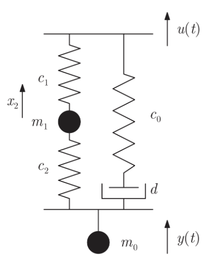
An example for a system with unstable zeros

Learning outcomes

By the end of this lecture, you should be able to

• Explain the different notions and forms of stability
• Analyze the stability properties of discrete-time dynamical systems using
  • Jury’s stability criterion
  • The Nyquist stability criterion
  • Lyapunov’s stability criterion

Stability tests

• The stability analysis of digital control systems is similar to the stability analysis of analog systems and known methods can be applied with some modifications

• For linear systems, we want to calculate the eigenvalues of the system matrix $Φ$

  \[\chi(z) := |zI - \Phi| = \det(zI - \Phi) \stackrel{!}{=} 0\]

  and check whether their absolute value is smaller than 1

• There are good numerical algorithms to compute the eigenvalues
  • In Python: numpy.linalg.eigvals(A)
  • in Matlab: eig(A)
• Other important methods include
  • Methods based on properties of characteristic polynomials (e.g., Jury’s criterion)
  • The root locus method
  • The Nyquist stability criterion
  • The Bode stability criterion
  • Lyapunov’s method

Jury’s stability criterion

• Explicit calculation of the eigenvalues of Φ cannot be done conveniently by hand for systems of order higher than 2

  \[\chi(z) := |zI - \Phi| = a_0 z^n + a_1 z^{n-1} + \ldots + a_{n-1} z + a_n \stackrel{!}{=} 0\]

• Jury’s stability criterion is the discrete-time analogue of the Routh-Hurwitz stability criterion:

  • The Jury stability criterion requires that the system poles are located inside the unit circle centered at the origin
  • The Routh-Hurwitz stability criterion requires that the poles are in the left half of the complex plane

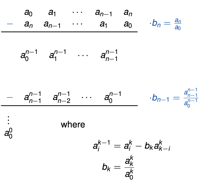
1st and 2nd rows are the coefficients of $\chi(z)$ in forward and reverse order, respectively

3rd row obtained by multiplying 2nd row by b_n and subtracting this from the 1st

4th row is the 3rd row in reverse order

The scheme is repeated until there are $2n+1$ rows, which includes a single term

Jury’s stability criterion
Suppose $a_0 > 0$. Then, the characteristic polynomial $\chi(z)$ has all its roots inside the unit circle if, and only if,
\(a_0^k > 0, \quad k = 0, 1, 2, \ldots, n-1.\) If no $a_0^k = 0$, then the number of negative $a_0^k$ is equal to the roots of $\chi(z)$ outside of the unit circle.

Example

• Consider a system with the following characteristic equation:

  \[\chi(z) = 3z^2 + 2z + 1.\]

Is the system stable?

\[\begin{array}{ccc|ccc} a_0 & a_1 & a_2 & 3 & 2 & 1 \\ a_2 & a_1 & a_0 & 1 & 2 & 3 \quad b_2 = \frac{1}{3} \\ \hline a_0^1 & a_1^1 & & 3 - 1 \cdot \frac{1}{3} = \frac{8}{3} & 2 - 2 \cdot \frac{1}{3} = \frac{4}{3} \\ a_1^1 & a_0^1 & & \frac{4}{3} & \frac{8}{3} \quad b_1 = \frac{4/3}{8/3} = \frac{1}{2} \\ \hline a_0^0 & & & \frac{8}{3} - \frac{1}{2} \cdot \frac{4}{3} = \mathbf{2} \end{array}\]

The system is stable: $a_0^0 > 0$, $a_1^0 > 0$, $a_0 > 0$
In fact, the roots can be easily solved directly: $-0.3333 \pm 0.4714j$

Example using symbolic calculations

• The Jury criterion can easily be used in the case of a small system, when a computer is not at hand
• Its real power lies in symbolic calculations: stability can be determined as a function of one or even more parameters
• For example, consider a system with characteristic equation

\[\chi(z) = z^2 + a_1 z + a_2\] \[\begin{array}{c c c | c c c} a_0 & a_1 & a_2 & 1 & a_1 & a_2 \\ a_2 & a_1 & a_0 & a_2 & a_1 & 1 \\ \hline a_0^1 & a_1^1 & & 1 - (a_2)^2 & a_1(1 - a_2) & \\ a_1^1 & a_0^1 & & a_1(1 - a_2) & 1 - (a_2)^2 & \\ \hline a_0^0 & & & 1 - (a_2)^2 - \frac{(a_1)^2 (1 - a_2)}{1 + a_2} & \end{array} \quad b_2 = \frac{a_2}{1} = a_2 \quad b_1 = \frac{a_1 (1 - a_2)}{1 - (a_2)^2} = \frac{a_1}{1 + a_2}\]

Example using symbolic calculations

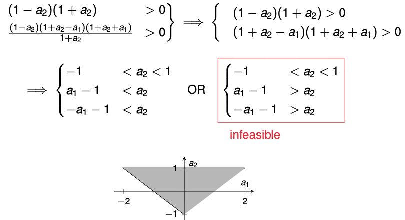
• The system is stable if
  \(\left\{ \begin{array}{l} 1 - (a_2)^2 > 0 \\ 1 - (a_2)^2 - \frac{(a_1)^2(1 - a_2)}{1 + a_2} > 0 \end{array} \right.\)

• Factoring differences of squares in the first inequality
  \(1 - (a_2)^2 = (1 - a_2)(1 + a_2) > 0\)

• Doing algebraic manipulations to the second inequality
  \(1 - (a_2)^2 - \frac{(a_1)^2(1 - a_2)}{1 + a_2} = \frac{(1 - a_2)(1 + a_2)^2 - (a_1)^2(1 - a_2)}{1 + a_2} = \frac{1 - a_2}{1 + a_2} \left[(1 + a_2)^2 - (a_1)^2 \right] = \frac{(1 - a_2)(1 + a_2 - a_1)(1 + a_2 + a_1)}{1 + a_2} > 0\)

• The set of inequalities can be simplified to (triangle rule):

Stability in the frequency domain

• The frequency response of $G(s)$ is $G(j\omega), \omega \in [0, \infty)$. It can be graphically represented
  • in the complex plane as the Nyquist curve, or,
  • as amplitude/phase curves as a function of frequency – Bode diagram
• Correspondingly, for a discrete-time system $H(z)$, the frequency response is $H(e^{j\omega}), \omega T_s \in [-\pi, \pi)$. This can also be graphically represented as discrete-time Nyquist curve or discrete-time Bode diagram

• Note that it is sufficient to consider the map in the interval $\omega T_s \in [-\pi, \pi)$ because the function $H(e^{j\omega})$ is periodic with period $\frac{2\pi}{T_s}$

• Consider, for example, the continuous-time system with transfer function
  \(G(s) = \frac{1}{s^2 + 1.4s + 1}\)

• ZOH sampling of the system with $T_s = 0.4$ gives the discrete-time system
  \(H(z) = \frac{0.066z + 0.055}{z^2 - 1.45z + 0.571}\)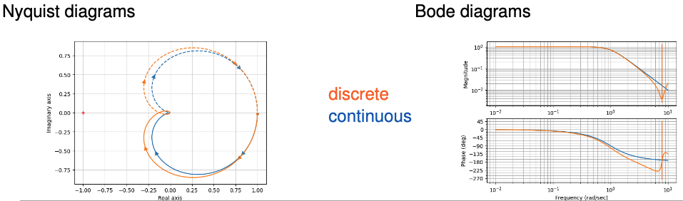

Nyquist diagram

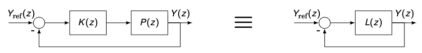
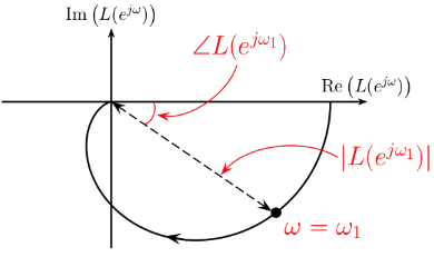
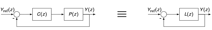
• Nyquist diagram: a plot of the open-loop frequency response of $L(z)$, with the imaginary part $\mathrm{Im}(L(e^{j\omega}))$ plotted against the real part $\mathrm{Re}(L(e^{j\omega}))$ on an Argand diagram (complex plane)

Recap from Lecture 3: how to find $L(e^{j\omega})$

• As we have already seen, a rational z-transform can be written as
  \(L(z) = c \frac{(z - \mu_1)(z - \mu_2) \ldots (z - \mu_M)}{(z - p_1)(z - p_2) \ldots (z - p_N)}\)

• To compute the frequency response of $L(e^{j\omega})$, we compute $L(z)$ at $z = e^{j\omega}$
• But $z = e^{j\omega}$ represents a point on the circle’s perimeter

• Let $A_i = \left

  e^{j\omega} - p_i \right

  $ and $B_i = \left

  e^{j\omega} - \mu_i \right

  $

\[\begin{aligned} |L(e^{j\omega})| &= |c| \frac{|e^{j\omega} - \mu_1| \, |e^{j\omega} - \mu_2| \ldots |e^{j\omega} - \mu_M|}{|e^{j\omega} - p_1| \, |e^{j\omega} - p_2| \ldots |e^{j\omega} - p_N|} \\ &= |c| \frac{B_1 B_2 \ldots B_M}{A_1 A_2 \ldots A_N}, \quad N \ge M \end{aligned}\]

\(\angle L(e^{j\omega}) = \angle (e^{j\omega} - \mu_1) + \angle (e^{j\omega} - \mu_2) + \ldots + \angle (e^{j\omega} - \mu_M) - \angle (e^{j\omega} - p_1) - \angle (e^{j\omega} - p_2) - \ldots - \angle (e^{j\omega} - p_N)\)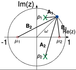

Discrete-time Nyquist stability criterion

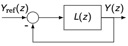
Definition: asymptotic stability of a feedback system
We say that the closed-loop system is asymptotically stable if the closed-loop transfer function $\frac{L(z)}{1+L(z)}$ is asymptotically stable.

• Closed-loop poles $\equiv$ poles of $\frac{L(z)}{1+L(z)} \equiv$ zeros of $1 + L(z)$
• This corresponds to all roots lying in the unit circle, i.e., if the characteristic equation has zeros outside the unit circle, the closed loop system is unstable

Nyquist plot

• We can assess the stability of the system by drawing the Nyquist diagram of $L(z)$
• The characteristic equation (whose zeros we usually compute to assess stability) is
  \(1 + L(z) \stackrel{!}{=} 0\)
• We now have the result that the open-loop Nyquist curve encircles the point $-1$ \(N = Z - P\) times clockwise
• $Z$ is the number of zeros of the characteristic equation outside the unit circle, $P$ the number of poles outside of the unit circle
• Zeros determine stability, so we need $Z = 0$
  $\Rightarrow$ Thus, for stability, we need $N = -P$

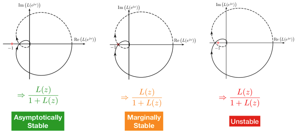
Discrete-time Nyquist stability criterion

Discrete-time Nyquist stability criterion

will be stable if, and only if, the number of encirclements $N$ of the point $-1$ by $L(e^{j\omega})$ as $\omega$ increases from 0 to $2\pi$ is equal to

\[N = -P\]

where:
$P$: # of poles of $\chi(z) : 1 + L(z)=0$ outside the unit circle, and clockwise encirclements count positive while a counterclockwise encirclement decreases $N$ by one.

Discrete-time Nyquist stability criterion

• The open-loop poles are the same as the poles of the characteristic equation
• The zeros of $\chi(z)$ determine the stability of the system
• If the characteristic equation has zeros outside the unit circle, then the closed-loop system is unstable
• Stability is thus obtained by setting $Z = 0$ and by demanding that the Nyquist curve encircles the point $-1\ P$ times counterclockwise
• The criterion becomes simple, if the open-loop pulse transfer function $L(z)$ has no poles outside the unit circle
• Then, the Nyquist curve must not encircle the point $-1$ at all

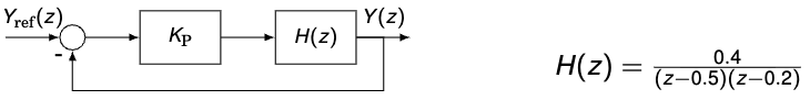
Example

• A discrete-time process ($T_s = 1$) is controlled with a proportional controller with $K_{\mathrm{P}}$

• We plot the Nyquist diagram with Python

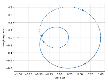
• By zooming in at the intersection with the real axis, the point is approximately $-0.4416$
• The magnitude can thus be multiplied with $\frac{1}{0.4416}$ to reach the critical point $-1$

• The controlled system is stable when \(K_{\mathrm{P}} < \frac{1}{0.4416} \approx 2.26\)

• Find the values of $K_P$ for which the system

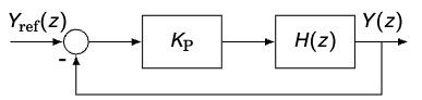
is stable with $H(z) = \frac{1}{z-2}$.

• Let’s start for $K_P = 1$. We have one unstable pole, so we need one counter-clockwise encirclement of $-1$

• $H \left( e^{j\omega} \right) = \frac{1}{e^{j\omega} - 2}$

• For $\omega = 0$: $H(0) = -1$

• For $\omega = \pi$: $H(j\pi) = -\frac{1}{3}$

$\Rightarrow$ The system is stable if

\[-1 < -\frac{1}{K} < -\frac{1}{3} \implies 1 < K < 3\]

Open-loop poles on the unit circle

Closing the plot: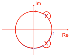

• To obtain a closed curve for the Nyquist plot (and hence correctly count the encirclements), it is customary to indent the path of $e^{j\omega}$ around the poles on the unit circle with a small semi-circular excursion outside the unit circle

• Then, the open-loop poles on the unit circle are counted as being stable in the stability criterion
• The “right turn” in the $z$-plane gives a “right turn” in the Argand diagram and a circular arc of large radius is produced

Asymptotes:

• If there is an open-loop pole of multiplicity one on the unit circle, then the Nyquist diagram will be asymptotic to a straight line as it tends to infinity
• It is possible to find the asymptote along which it tends
• Suppose $H(z)$ has a pole at $z = 1$, i.e.,
  \(H(z) = \frac{1}{z-1} F(z)\) where $F(z)$ has no poles at $z = 1$
• Then, for $z \approx 1$, expand $F(z)$ in a Taylor series to give
  \(H(z) = \frac{1}{z-1}\left(F(1) + (z-1)F'(1) + \frac{1}{2}F''(z)(z-1)^2 + \ldots \right) \approx \frac{F(1)}{z-1} + F'(1)\)

Open-loop poles on the unit circle

• But
  \(\frac{1}{e^{j\omega}-1} = \frac{1}{e^{j\frac{\omega}{2}}\left(e^{j\frac{\omega}{2}} - e^{-j\frac{\omega}{2}}\right)} = \frac{e^{-j\frac{\omega}{2}}}{2j\sin\left(\frac{\omega}{2}\right)} = \frac{\cos\left(\frac{\omega}{2}\right) - j \sin\left(\frac{\omega}{2}\right)}{2j \sin\left(\frac{\omega}{2}\right)} = -\frac{1}{2} - \underbrace{\frac{j}{2 \tan\left(\frac{\omega}{2}\right)}}_{\text{large as } \omega \to 0}\)

• Hence
  \(H(e^{j\omega}) \approx \underbrace{-\frac{1}{2}F(1) + F'(1)}_{\text{constant real part}} - j \frac{F(1)}{2 \tan\left(\frac{\omega}{2}\right)}\)

• For multiple poles on the unit circle the asymptotic behavior is more complex and requires more terms in the Taylor series expansion

Gain and phase margins

• $L(e^{j\omega})$ being close to $-1$ without encircling it is undesirable for 2 main reasons:
  1. It implies that a closed-loop pole is close to the imaginary axis and the closed-loop system will oscillate
  2. If our plant $P(z)$ is the transfer function of an inaccurate model, the “true” Nyquist diagram might actually encircle $-1$

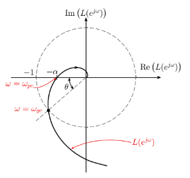
• The gain margin (GM) is a measure of how much the gain can be increased before the closed-loop system becomes unstable
  \(\text{GM} = \frac{1}{\alpha} = \frac{1}{\left| L\left(e^{j \omega_{pc}}\right) \right|}\)

• The phase margin (PM) is a measure of how much phase lag can be added before the closed-loop system becomes unstable
  \(\text{PM} = \theta = \pi + \angle L\left(e^{j \omega_{gc}}\right)\)

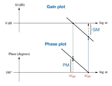
Gain and phase margins via Bode plots

• ■ Phase crossover frequency $\omega_{pc}$: frequency at which the phase equals $180^\circ$
• ■ Gain crossover frequency $\omega_{gc}$: frequency at which the magnitude equals 1

Lyapunov’s stability theory

• A useful tool for determining the the stability of linear and nonlinear dynamical systems
• Allows to guarantee asymptotic stability, regions of stability, etc.
• Main idea: introduce a generalized energy function, called the Lyapunov function, which is zero at the equilibrium and positive elsewhere

Some history

Historical notes

• Aleksandr Mihailovich Lyapunov developed the theory for differential equations in 1900, but the corresponding theory has also been developed for difference equations
• Lyapunov is well-known for his development of the stability theory of a dynamical system, as well as for his contributions to mathematical physics and probability theory
• The theory passed into oblivion, until N. G. Chetaev realized the magnitude of the discovery made by Lyapunov
• The interest in it skyrocketed during the Cold War period when it was found to be applicable to the stability of aerospace guidance systems which typically contain strong nonlinearities not treatable by other methods

Lyapunov’s stability theory

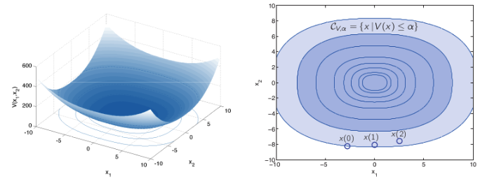
• Geometric illustration of Lyapunov’s theorem:
  • Lyapunov function $V(x)$ (left)
  • Level curves for Lyapunov function $V(x)$ in the 2-dimensional case (right). All level curves encircle the origin and do not intersect any other level curve
• Stability:
  • Once the state enters a level set, it does not leave. Bounded level sets ensure bounded trajectories (stability)
  • The equilibrium will be asymptotically stable if we can show that the Lyapunov function decreases along the trajectories of the system

Lyapunov function

• $V(x)$ is a Lyapunov function for the system
  \(x_{k+1} = f(x_k), \quad f(0) = 0\) if
  1. $V(x)$ is continuous in $x$ and $V(0) = 0$
  2. $V(x) \geq 0$ for all $x$
  3. $\Delta V(x) = V(x_{k+1}) - V(x_k)$ is negative definite
• Condition 3 implies that the dynamics of the system is such that the solution always moves toward curves with lower values

Stability theorem of Lyapunov

• From the geometric interpretation: the existence of a Lyapunov function ensures asymptotic stability
• The following theorem is a precise statement of this fact

Lyapunov’s stability theorem
The solution $x_k = 0$ is asymptotically stable if there exists a Lyapunov function to the system
\(x_{k+1} = f(x_k), \quad f(0) = 0\)
Further, if
\(0 < \phi(\|x\|) < V(x)\)
where $\phi(|x|) \to \infty$ as $|x| \to \infty$, then the solution is asymptotically stable for all initial conditions

• Main obstacle to using the Lyapunov theory is finding a suitable Lyapunov function

Application to linear systems

• For the linear system
  \(x_{k+1} = \Phi x_k, \quad x_0 = \alpha\)
  we can use the quadratic Lyapunov function
  \(V(x) = x^{\mathrm{T}} P x\)

• The increment of $V$ is then given by
  \(\begin{aligned} \Delta V(x) &= V(x_{k+1}) - V(x_k) = V(\Phi x_k) - V(x_k) \\ &= x_k^{\mathrm{T}} \Phi^{\mathrm{T}} P \Phi x_k - x_k^{\mathrm{T}} P x_k \\ &= x_k^{\mathrm{T}} \left( \Phi^{\mathrm{T}} P \Phi - P \right) x_k \\ &= - x_k^{\mathrm{T}} Q x_k \end{aligned}\)

• For $V$ to be a Lyapunov function it is necessary and sufficient that there exist positive definite matrices $P$ and $Q$ that satisfy the Lyapunov equation
  \(\Phi^{\mathrm{T}} P \Phi - P = -Q\)

• There is always a solution to the Lyapunov equation when the linear system is stable
• P is positive definite if Q is positive definite
  → Choose a positive definite matrix Q and solve the Lyapunov equation
  → If the solution P is positive definite the system is asymptotically stable
• In Python: scipy.linalg.solve_discrete_lyapunov(Φ, Q)
• In MATLAB: dlyap(Φ, Q)
• Example
  • Consider the system
    \(x_{k+1} = \begin{pmatrix} 0.4 & 0 \\ -0.4 & 0.6 \end{pmatrix} x_k\)
  • Choose $Q = \begin{pmatrix} 1 & 0 \ 0 & 1 \end{pmatrix}$
  • Solve Lyapunov equation:
    \(P = \begin{pmatrix} 1.19 & -0.25 \\ -0.25 & 2.05 \end{pmatrix}\)

Summary

• We have studied 3 ways of checking stability for discrete-time systems
• Jury’s stability criterion
  ✓ Can handle systems of order higher than 2
  ✓ Symbolic calculations can give us a sense of robustness
  ✗ Gets very tedious to do by hand for higher order systems
• Nyquist stability criterion
  ✓ Graphical representation with criterion that is easy to check from the plot
  ✓ Gain and phase margin are informative for robustness
  ✗ Difficult to draw Nyquist plot when we don’t have a computer
• Lyapunov’s stability criterion
  ✓ General approach that works also for nonlinear systems
  ✓ For linear systems, we can use quadratic Lyapunov equation
  ✗ Solving Lyapunov equation by hand is difficult even for linear systems
  ✗ For nonlinear systems, we need to guess Lyapunov function

Learning outcomes

By the end of this lecture, you should be able to

• Explain the different notions and forms of stability
• Analyze the stability properties of discrete dynamical systems using:
  • Jury’s stability criterion,
  • The Nyquist stability criterion, and
  • Lyapunov’s stability criterion

Exam

• Content: everything until and including state-space representations (i.e., content of today’s lecture is not relevant)
• There will be exercises where you need to calculate something similar to exercise/homework tasks
• There will also be understanding questions (why is the solution like that? what would change if . . . ?)
• Calculators are not allowed (and not needed)
• You can handwritten, one-sided A4 page on which you can write whatever you feel might help you during the exam
• We will check the sheets at the beginning of the exam, so please make sure you don’t write more than 1 A4 page
• You should know (or write on your sheet) the general rules of Laplace and z-transforms, like, what is a derivative/prediction in the Laplace/z-domain. If more complicated transforms are required, like the transform of a sin, we will give them.
• The exam will be Wednesday, 15.10., AS2, 09:00 – 12:00