2025-09-01-ELEC-E8101 - Digital and Optimal Control 1
Digital and Optimal Control 1
Preliminaries
Digital and Optimal Control 1 Introduction
Office number: 2569, Maarintie 8
dominik.baumann@aalto.fi
Sep. 01, 2025
Learning outcomes
By the end of this lecture, you should be able to
- Explain the importance of feedback control in general and digital control in particular
- List the advantages and disadvantages of digital control
- Explain the implications of converting continuous-time into discrete-time models
- Derive and use the properties of Laplace transforms to represent continuous-time systems
A simple example: controlling the speed of a car
- We have a car (we call it the system or the plant)
- We have the motor torque and brakes (we call it the input signal)
- We have the speed (we call it the output signal)
- We have the feet that press the gas and brake pedals (we call it the controller)
- We have a reference speed (we call it the reference signal)
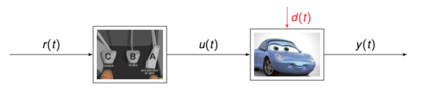
- The controller computes the input signal $u(t)$ that lets the output signal $y(t)$ follow the reference signal $r(t)$
- Solution without feedback ( open-loop control ) relies on constant conditions
But what happens if the road slope changes (disturbances)?
- We need to adapt to slope changes (disturbances )
- So, we need some information about the speed feedback
- The controller takes slope changes (disturbances) into account by observing the speed (feedback )
- This solution is with feedback (closed-loop control)
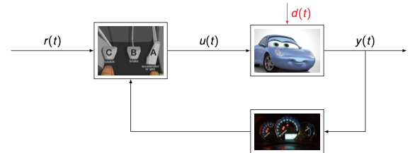
- $r(t)$ input to the controller (left block: clutch, brake, accelerator)
- Controller output $u(t)$ to the car (middle block: blue car)
- Disturbance $d(t)$ acting on the car (red arrow)
- Output $y(t)$ is the speed observed (right block: speedometer)
Feedback path from output back to controller
- Ideally, we want to automate this process
→ Automatic control - In cars, this is often implemented in the form of cruise control systems
Why do we need feedback control systems?
Open-loop system
1
reference point → Controller → Plant → plant output
- A controller can be adjusted to give the right output
- Works provided there are no disturbances!

Closed-loop systems
- Deviations from the reference point are corrected automatically
Application areas of control engineering
- Automotive, aeronautics & aerospace engineering
- Process control (chemical, pharmaceutical, . . . )
- Robotics, manufacturing
- Power electronics, power networks
- Telecommunications
- Financial engineering
- . . .
Applications of feedback control systems
Domestic applications
Regulated voltage and frequency of electric power, thermostat control of refrigerators, temperature and pressure control of hot water, pressure of fuel gas, autofocus of digital cameras, . . .Industrial applications
Process regulators, process and oven regulators, steam and air pressure regulators, gasoline and steam engine governors, motor speed regulators, . . .Transportation systems
Speed control of airplane engines, control of engine pressure, instruments in the pilot’s cabin contain feedback loops, instrument-landing system, . . .Automobiles
Thermostatic cooling system, steering mechanisms, the gasoline gauge, and collision avoidance, idle speed control, antiskid braking, . . .Scientific applications
Measuring instruments, analog computers, electron microscope, cyclotron, x-ray machine, space ships, moon-landing systems, remote tracking of satellites, . . .
From analog to digital control
- Classical and modern control theory for continuous-time control systems has revolutionized industrial processes (a few years ago)
Treating systems in continuous time in theory requires immediate feedback, e.g., when the feedback loop is implemented in hardware
- In practice, nowadays, controllers are typically implemented on microprocessors
Why are we interested in digital control?
- Digital computers and microprocessors offer tremendous amount of flexibility and versatility in the design approach
- For some applications, better system performance can be achieved with digital control system design
- Digital control uses digital communication:
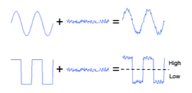
- More reliable due to its improved noise immunity
- Better resolution when representing numbers
Disadvantages/problems of digital control?
- Complicated controllers implemented in software may have software errors
- Most control processes are analog in nature:
- Signal from digital controller → converted to analog (D/A converter) – hold
- ?
- Signal to the digital controller → converted to digital (A/D converter) – sampling
- Converting signals can cause information loss
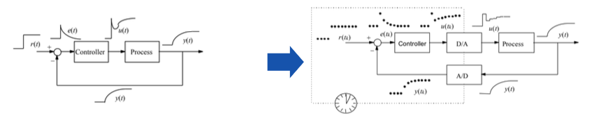
- Signal from digital controller → converted to analog (D/A converter) – hold
- A/D and D/A converters introduce some time-delay → performance objectives may be difficult to achieve
- Mathematical analysis sometimes more complex
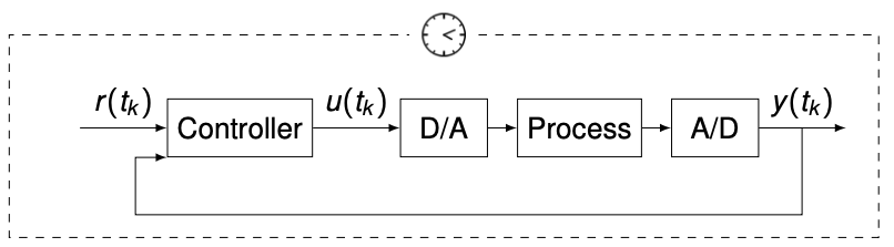
Discrete-time controller design
There are 2 main design approaches
Discretize the analog controller
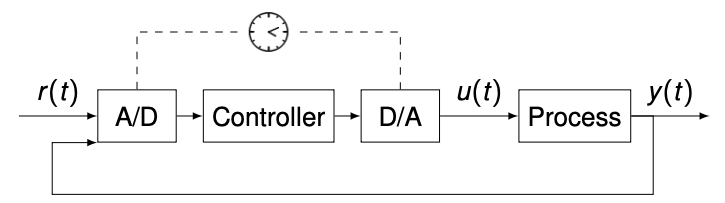
Discretize the process and do the entire design in discrete time
To think about…
- The system contains both analog and discrete signals (hybrid system). How do you treat these kinds of systems analytically?
- Are the traditional time-domain and frequency-domain methods useful in this context? Can they be modified?
- How do you design digital controllers? What should be taken into account in the implementation?
- Is it so that a digital controller only imitates the corresponding analog controller and the result is somewhat worse then (due to losing information in discretization)?
- Do discrete-time systems have properties that the corresponding analog systems do not have?
Example: controlling the arm of a disk drive
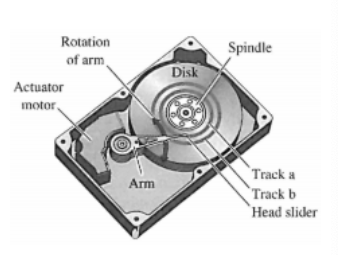
The dynamics of relating the position y of the arm to the voltage u of the drive amplifier is approximately described by the transfer function
\[G(s) = \frac{k}{Js^2}\]where k is a constant and J the inertia.
A servo-controller is given by
\[U(s) = K \frac{b}{a} U_c(s) - K \frac{s + b}{s + a} Y(s),\]where $u_c$ is the reference signal.
- Discretize the analog servo controller to obtain a digital one!
- To obtain a digital controller, the servo controller is first re-written:
- Transforming it to the time domain, we obtain
- We also need an expression for $x(t) $
- We know
- We can rewrite this
\(sX(s) + aX(s) = (a - b) Y(s)\) \(\frac{\text{d} x(t)}{\text{d} t} + a x(t) = (a - b) y(t)\)
- From the previous slide, we have
- To obtain a discrete-time controller, we approximate the derivative:
- Hence, we obtain the following approximated discrete controller:
\(x(t_k + T_s) - x(t_k) = T_s(-ax(t_k) + (a - b)y(t_k))\) 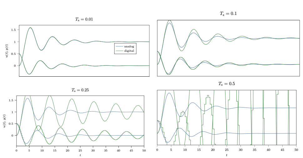
- Deadbeat control: bring output to steady-state in minimal number of time steps
- Control strategy used has a somewhat similar form as the previous controller
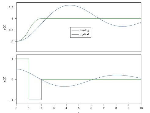
- Settles much quicker than continuous-time controller
- Output reaches desired value without overshoot
- We will study this concept in Lecture 9
- Such a control scheme cannot be obtained with a continuous-time controller!
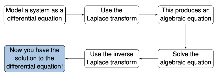
Recap: Laplace transform
- The Laplace transform is very similar to the Fourier transform
- The Laplace transform often simplifies the analysis of continuous-time systems
- For example, the Laplace transform transforms differential equations into algebraic equations and convolutions into multiplications
For these reasons, analog systems are often designed and analyzed using the Laplace transform
- Advantages
- Provides a complete solution
- Much less time is involved in solving the differential equations
- Initial conditions are automatically considered in the transformed equations
- It provides a systematic and routine solution for differential equations
Definition of the Laplace transform
Laplace transform
The Laplace transform $X(s)$ of a function $x(t)$, for $t > 0$, is defined by \(\mathscr{L} \{ x(t) \} := X(s) = \lim_{T \to \infty} \int_{\tau=0}^{T} x(\tau) e^{-s\tau} \, \mathrm{d}\tau,\) where $s$ is a complex number.
- There are 3 main tools for obtaining Laplace transforms
- The definition
- Laplace transform properties
- Lists of transforms of known functions
- In what follows, we will study the 3 approaches
From the definition
Here, we use the definition (with slight abuse of notation) directly
\(X(s) = \int_{t=0}^\infty x(t) e^{-st} dt\)Example 1: consider the function $x(t) = 1$:
\(\mathscr{L}\{1\} = \int_0^\infty e^{-st} dt = \left[-\frac{1}{s} e^{-st}\right]_0^\infty = \frac{1}{s}\)Example 2: consider the function $x(t) = e^{at}$, where $a$ is a constant:
\(\mathscr{L}\{e^{at}\} = \int_0^\infty e^{at} e^{-st} dt = \int_0^\infty e^{-(s-a)t} dt = \left[-\frac{1}{s-a} e^{-(s-a)t}\right]_0^\infty = \frac{1}{s-a}\)Example 3: consider the function $x(t) = t$ (for a reminder on integration by parts, see the appendix):
\(\mathscr{L}\{t\} = \int_0^\infty t e^{-st} dt = \left[-\frac{1}{s} t e^{-st}\right]_0^\infty + \int_0^\infty \frac{1}{s} e^{-st} dt = \frac{1}{s^2}\)From properties of the Laplace transform
Linearity
\(\mathscr{L}\{af(t) + bg(t)\} = a\mathcal{L}\{f(t)\} + b\mathcal{L}\{g(t)\}\)
Derivative
\(\mathscr{L}\{f'(t)\} = sF(s) - f(0)\)
Frequency shifting
\(\mathscr{L} \left\{ e^{at} f(t) \right\} = F(s - a)\)
Convolution
\(\mathscr{L}\{(f * g)(t)\} = F(s)G(s)\)
De Moivre’s
\(\mathscr{L}\{ \cos(at) + j \sin(at) \} = \mathscr{L} \left\{ e^{jat} \right\} = \frac{1}{s - ja} = \frac{s}{s^2 + a^2} + j \frac{a}{s^2 + a^2}\)
Final value theorem
\(\lim_{t \to \infty} f(t) = \lim_{s \to 0} sF(s)\)
Initial value theorem
\(f(0) = \lim_{s \to \infty} sF(s)\)
From a list of known Laplace transforms
| Waveform: $g(t)$ (defined for $t \geq 0$) | Laplace Transform: $G(s) = \mathcal{L}{g(t)} = \int_0^\infty g(t)e^{-st}dt$ |
|---|---|
| $\delta(t)$ impulse | 1 |
| $u(t)$ unit step | $\frac{1}{s}$ |
| $t^n$ | $\frac{n!}{s^{n+1}}$ |
| $e^{-at}$ | $\frac{1}{s+a}$ |
| $\sin(\omega_0 t)$ | $\frac{\omega_0}{s^2 + \omega_0^2}$ |
| $\cos(\omega_0 t)$ | $\frac{s}{s^2 + \omega_0^2}$ |
| $\sinh(\omega_0 t)$ | $\frac{\omega_0}{s^2 - \omega_0^2}$ |
| $\cosh(\omega_0 t)$ | $\frac{s}{s^2 - \omega_0^2}$ |
| $e^{-at}A \cos(\omega_0 t) + B \sin(\omega_0 t)$ | $\frac{A(s+a) + B\omega_0}{(s+a)^2 + \omega_0^2}$ |
| $e^{-at}g(t)$ | $G(s + a)$ shift in $s$ |
| $g(t - \tau)u(t - \tau)$ where $\tau \geq 0$ | $e^{-s \tau} G(s)$ shift in $t$ |
| $t g(t)$ | $-\frac{d}{ds}G(s)$ |
| $\frac{dq}{dt}$ differentiation | $sG(s) - q(0)$ |
| $\frac{d^n q}{dt^n}$ | $s^n G(s) - s^{n-1} q(0) - s^{n-2} \left(\frac{dq}{dt}\right)_0 - \ldots - \left(\frac{d^{n-1} q}{dt^{n-1}}\right)_0$ |
| $\int_0^t g(\tau)d\tau$ integration | $\frac{G(s)}{s}$ |
| $g_1(t) * g_2(t)$ convolution | $G_1(s) G_2(s)$ |
| $\quad = \int_0^t g_1(t - \tau) g_2(\tau) d\tau$ |
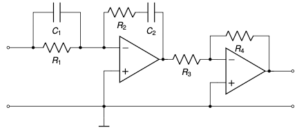
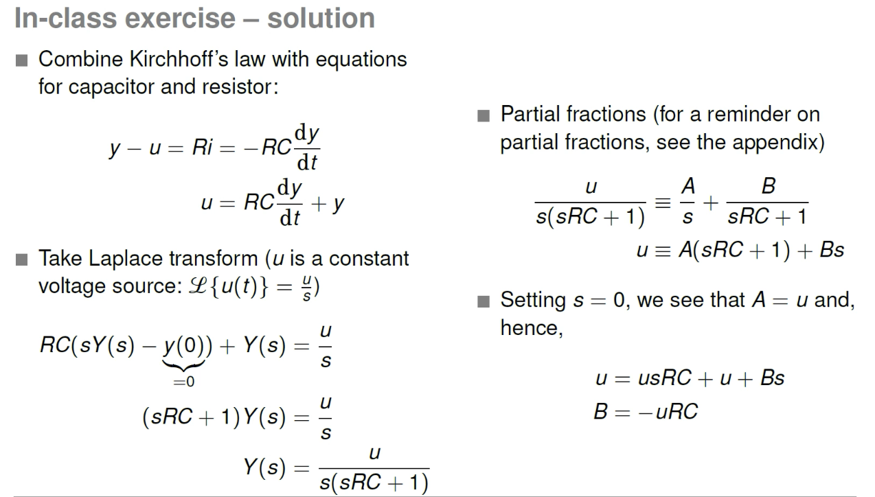
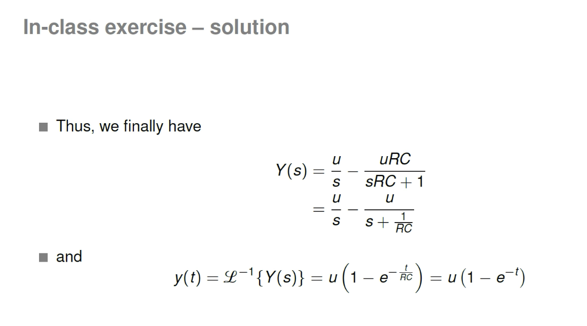
In-class exercise
Find the voltage y of the capacitor in the circuit below, provided $y(0) = 0$. 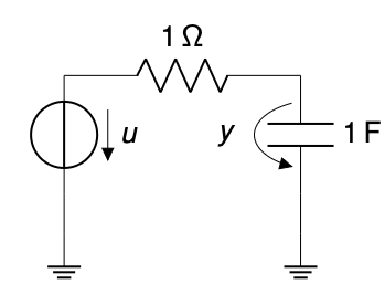
Reminder
- Capacitor:
- Resistor:
(Note: The circuit diagram shows a voltage source $u$, a 1 Ω resistor, and a 1 F capacitor with voltage $y$.)
Laplace transform – closing remarks
- The Laplace transform can help with analyzing continuous-time systems
- It is not applicable to discrete-time systems!
- For discrete-time system, a similar transform exists: the z-transform
- More on this in the next lecture
Learning outcomes
By the end of this lecture, you should be able to
- Explain the importance of feedback control in general and digital control in particular
- List the advantages and disadvantages of digital control
- Explain the implications of converting continuous-time into discrete-time models
- Derive and use the properties of Laplace transforms to represent continuous-time systems
Appendix
Integration by parts
- Recall the chain rule for differentiation
- If we integrate both sides with respect to $t $, we get
- Rearranging
- This gives us a useful way of integrating products
Partial fractions
- Many equations involving rational expressions can be solved easier if partial fraction decomposition is done beforehand
Assume a rational expression of the form
\[f(s) = \frac{P(s)}{Q(s)}\]where both $P(s)$ (numerator) and $Q(s)$ (denominator) are polynomials and the degree of $P(s)$ is smaller than the degree of $Q(s)$
- Note: partial fraction decomposition can only be done if the degree of the numerator is strictly less than the degree of the denominator
Partial fractions
| Factor in denominator | Term in partial fraction decomposition |
|---|---|
| $(as + b)$ | $\rightarrow \frac{A}{as+b}$ |
| $(as + b)^k$ | $\rightarrow \frac{A_1}{as+b} + \frac{A_2}{(as+b)^2} + \cdots + \frac{A_k}{(as+b)^k}$ |
| $(as^2 + bs + c)$ | $\rightarrow \frac{As + B}{as^2 + bs + c}$ |
| $(as^2 + bs + c)^k$ | $\rightarrow \frac{A_1 s + B_1}{as^2 + bs + c} + \frac{A_2 s + B_2}{(as^2 + bs + c)^2} + \cdots + \frac{A_k s + B_k}{(as^2 + bs + c)^k}$ |
Examples:
\[\frac{P(s)}{(as^{2} + bs + c)(ds + e)} \rightarrow \frac{As + B}{as^{2} + bs + c} + \frac{C}{ds + e}\] \[\frac{P(s)}{(as + b)^{2}(ds + e)} \rightarrow \frac{A}{as + b} + \frac{B}{(as + b)^2} + \frac{C}{ds + e}\]1. 什么是拉普拉斯变换?
拉普拉斯变换(Laplace Transform)是一种 积分变换工具,作用是把一个时间函数(随 $t$ 变化的信号,比如电路里的电压、电流)转化为复频域(以复数变量 $s$ 表示)的函数。
数学定义:
\[X(s) = \mathcal{L}\{x(t)\} = \int_0^\infty x(t) e^{-st} \, dt, \quad s \in \mathbb{C}.\]这里:
- $x(t)$:原始时间信号;
- $X(s)$:变换后的函数(频域表达式)。
2. 为什么要用它?
它的最大好处是:
把微分方程变成代数方程。
- 时间域:$\frac{dy}{dt}$ 很难算;
- $s$-域:$\mathcal{L}{\frac{dy}{dt}} = sY(s) - y(0)$,变成乘法。
👉 所以工程里(电路、控制系统)经常用它来解一阶/二阶的微分方程。
3. 变换之后是不是还需要反变换?
对的!
- 正变换(Laplace Transform):$x(t) \to X(s)$,方便我们解方程。
- 反变换(Inverse Laplace Transform):$X(s) \to x(t)$,回到时间域,得到我们真正想要的解。
符号写作:
\[x(t) = \mathcal{L}^{-1}\{X(s)\}.\]举个例子:
\[X(s) = \frac{1}{s} \quad \Rightarrow \quad x(t) = 1 \quad (t \ge 0).\]这就说明 $\frac{1}{s}$ 在 $s$-域里对应“阶跃函数”。
4. 用在电路题里的流程
像你那道 RC 电路题,步骤就是:
- 写电路的微分方程;
- 拉普拉斯变换,得到关于 $Y(s)$ 的代数方程;
- 解出 $Y(s)$;
- 反拉普拉斯变换,得到最终的时间函数 $y(t)$。
✅ 小总结:
- 拉普拉斯变换:时间函数 → 复频域函数;
- 它能让“微分方程”变成“代数方程”;
- 解完后必须 反变换 才能得到最终的时间解。