IML L4.1 Learning Curves

Learning Curves

Using polynomial features for this dataset

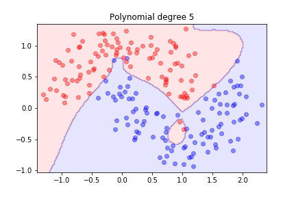
we achieved a good separation, but we wondered how well the model might generalise.

Testing the model

The data was generated according to a fixed probability density. We can produce a larger set and see how well the model does on new examples.

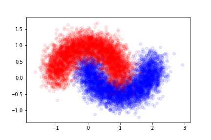
We will call this set the validation set here.

As we increase the polynomial degree the error on the training set decreases

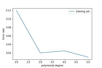
The error on the test set decreases at first but then increases again!

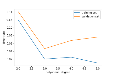
This is overfitting: the model learns the noise in the training set rather than the features of the underlying probability density.

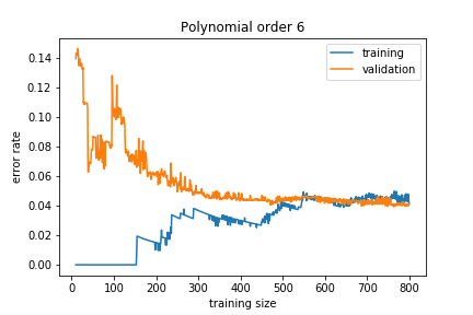
Learning curve

We can get insights into how the model is learned by looking at the learning curve.

It plots the error rate (the number of mis-classifications divided by the total number of samples) on the training set and on the validation set as a function of the number of data samples in the training set.

If the model is about right for the amount of training data we have we get

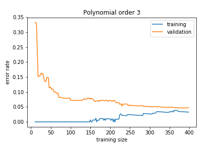
The training and validation sets converge to a similar error rate.

If the model is too simple, we get

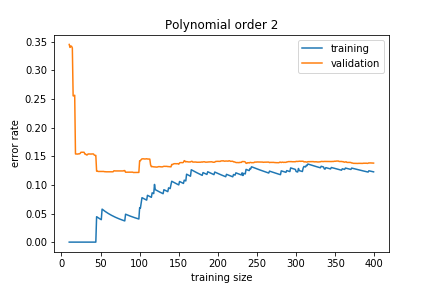
The training and validation errors converge, but to a high value because the model is not general enough to capture the underlying complexity. This is called underfitting.

If the model is too complex, we get

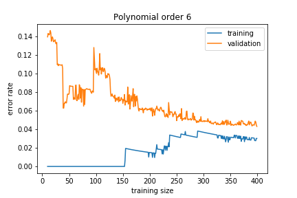
The training error is much smaller than the validation error. This means that the model is learning the noise in the training sample and this does not generalise well. This is called overfitting

Adding more training data reduces the overfitting: