IML L4.3 Regularisation

Regularisation

We can prevent a too general model from overfitting through regularisation.

We modify the loss function to include a penalty for too high parmeter:

\[J_{pen}(X,y.\vec w) = CJ(X,y,\vec w)+ \frac{1}{2}\vec w \cdot \vec w\]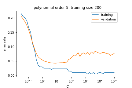

small values of CC means strong regularisation, large values of CC means weak regularisation.

1D regression example

We now look at a one-dimensional example. Say we have the relationship

\[{y=y(x)=7-8x-\frac12x^2+\frac12x^3+\epsilon}\]

where ϵϵ is gaussian noise of average 0 and unit variance.

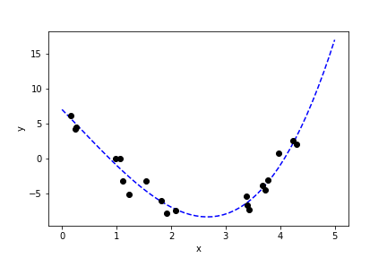
We can fit the data using polynomials of different order kk:

The fit is minimizing the least square objective:

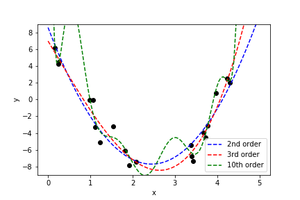
\[{J(x,y,w)=\sum_{i}\left(p_{w}(x^{(i)})-y^{(i)}\right)^{2};,\quad p_{w}(x)=\sum_{i=0}^{k}w_{i}x^{i}}\]

The third order fit gets close to the right coefficients:

A second order fit is not too bad:

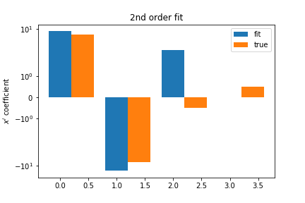
The 10th order polynomial is clearly overfitting, the polynomial coefficients are very large:

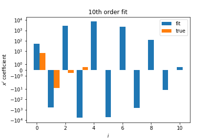
Large values and large cancellations between coefficients is a sign of overfitting.

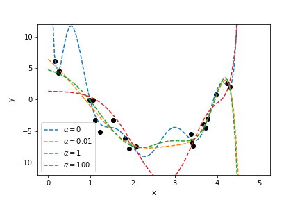
We can prevent large values of the coefficients if we modify the objective:

\[{J_{pen}(x,y,w,a)=J(x,y,w)+a\frac{1}{2}\sum_{i=0}^{k}w_{i}^{2}}\]

As we have seen for the SVM loss function we have two terms in the loss function that push ther result in opposite and conflicting directions. Small values of $\alpha$ do not change the objective function much and correspond to mild regularisation. Large values of $\alpha $ impose a stronger constraint on the size of the coefficients, meaning more regularisation.

This is called ridge regression.

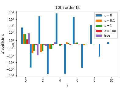
The regularised coefficients are a lot smaller then the unregularised ones:

Training/Validation/Test sets

In a normal problem we have no access to the underlying probability

• we need to separate our training data into a set for training and a set for validation
• the validation set is used to set the hyperparameters of the learning algorithm
• it is common to also have a “test” set set appart to check the algorithm on data not used for training or hyperparameter optimisation.

Cross validation

It is often the case that we do not have much labelled data and keeping a significant portion of it for hyperparameter optimisation often feels like a waste.

We can use a technique called cross-validation to perform validation without loosing too much of the training set.

In k-fold cross-validation we partition the data sample randomly into kk subsamples. For each subsample we train our model on the remaining subsamples and use the subsample we chose to validate the model. This will give a set of kk estimates of the model parameters. We can use these to

• obtain an estimate of the uncertainty of the model parameters
• estimate how well the model is going to generalise