IML L5.1 Neural networks

https://miscada-ml-2425.notes.dmaitre.phyip3.dur.ac.uk/assets/presentations/lecture-5/lecture-5.slides.html#/33

Neural networks

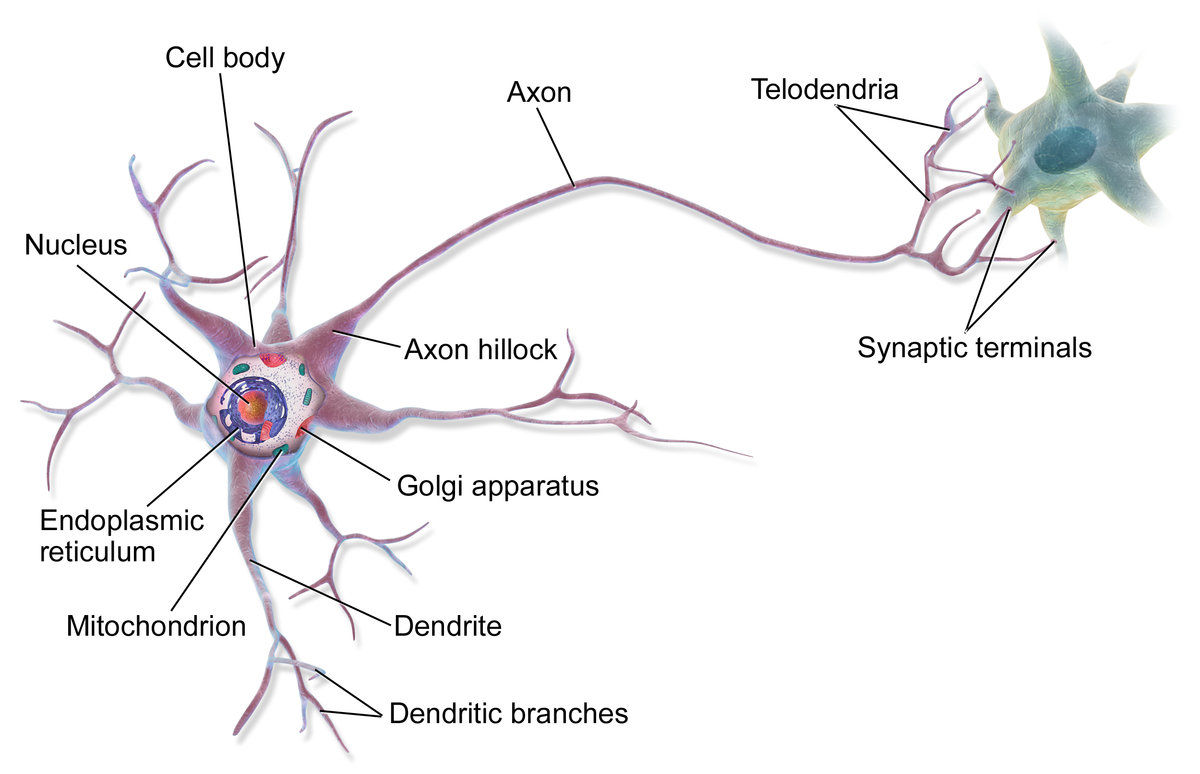
Neutral networks started as an attempt to model the human brain. It is composed of neurones

• Consist of layers of interconnected nodes called neurons .
• Each neuron processes input and passes the output to the next layer.
• Capable of learning complex patterns from data.
• Used in various domains like computer vision, natural language processing, and more.

The model for a neuron was the perceptron:

Models a single neuron. 模拟单个神经元。

Performs binary classification. 执行二元分类。

Mathematically, the perceptron computes: 感知器计算

\[z = w_0 + \vec w \cdot \vec x; \ \ \ \ \ output = \phi(z)\]

$\vec x = $ input vector 输入向量

$\vec w=$ weight vector 权重向量

$w_0=$ bias term 偏置项

$\phi(z)=$ activate function 激活函数

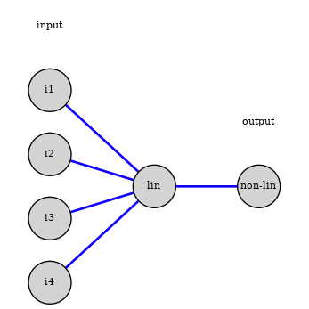
This is the model of a modern unit in a neural network:

• linear combination of inputs units
• non-linear function to generate the unit’s value, called activation function

The perceptron learning rule updates weights based on the error: 感知器学习规则根据错误更新权重： \(w_j \leftarrow w_j + \eta(y-\hat y)x_j\) where: 在哪里:

• $\eta$ = learning rate. 学习率。
• $y$ = true label.
• $\hat y$ = predicted label.

Limitations of the Perceptron 感知器的局限性

The perceptron has significant limitations: 感知器有显著的局限性：

• Can only solve linearly separable problems. 只能解决线性可分问题。
• Cannot model complex, non-linear decision boundaries (e.g., XOR problem). 无法建模复杂的非线性决策边界（例如，异或问题）。
• Limited representational capacity. 有限的表征能力。
• Led to the development of multi-layer networks to overcome these limitations. 导致了多层网络的发展以克服这些限制。

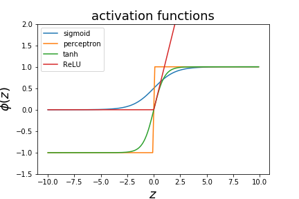
Non-linear activation functions

There are different decision functions that can be used.

• the perceptron used a step function
• logistic regression uses the sigmoid function
• one can also use $\phi(z) = tanh(z)$ as a decision function
• various variations on the hinge function (ReLU)

Network architectures

Neural networks are build by connecting artificial neurons together.

They can be used for classification or regression. Here we will consider the classification case.

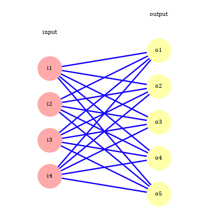
Single layer network

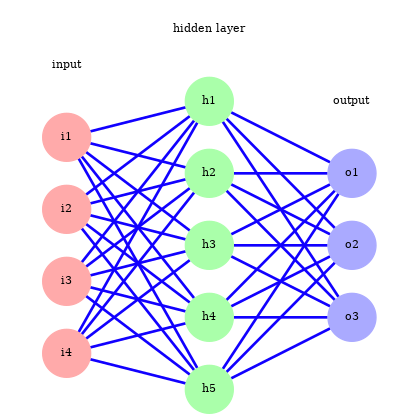
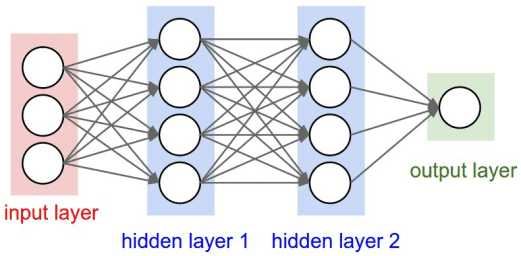
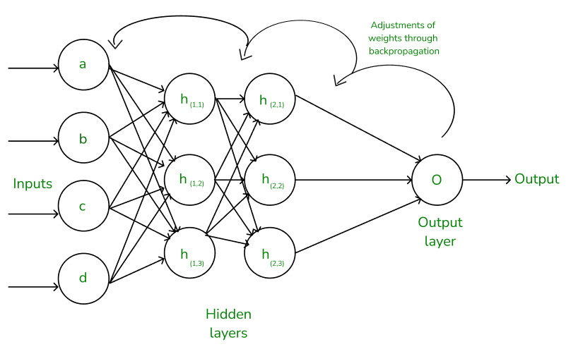
Multi layer network

Also known as Multi-Layer Perceptrons (MLPs). 也被称为多层感知器（MLPs）。

• Consist of an input layer, one or more hidden layers, and an output layer. 由一个输入层、一个或多个隐藏层和一个输出层组成。
• Hidden layers enable the network to learn complex, non-linear patterns. 隐藏层使网络能够学习复杂的非线性模式。
• Universal approximation theorem: MLPs can approximate any continuous function. 通用逼近定理：MLP 可以逼近任何连续函数。

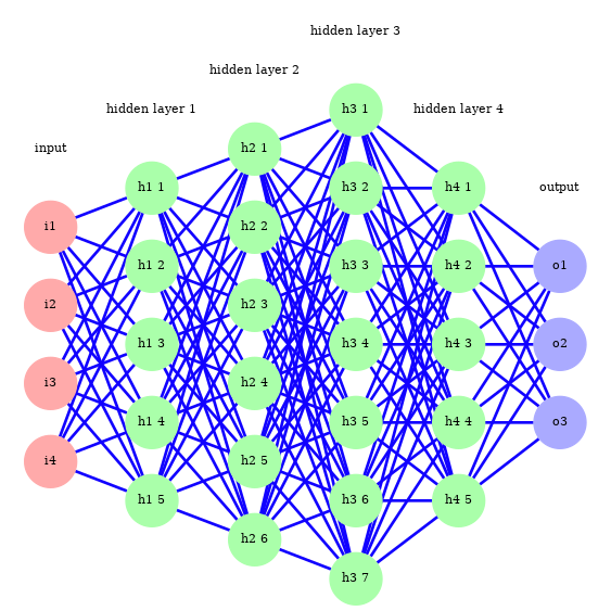
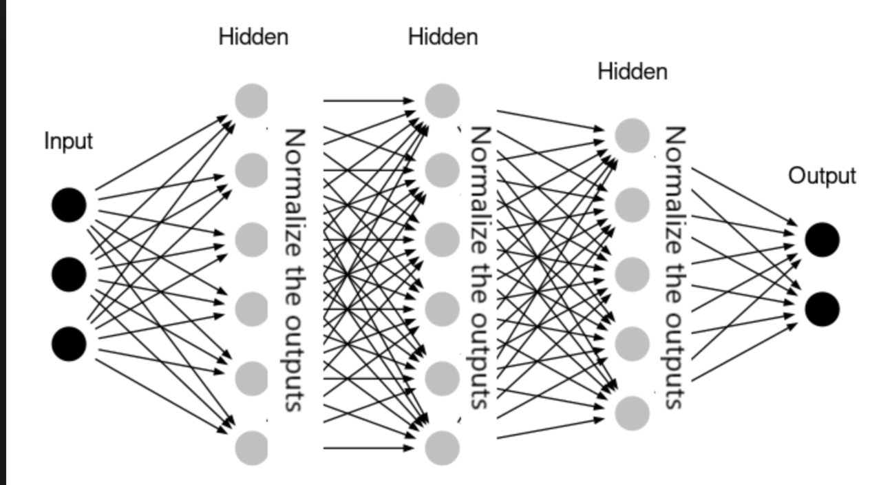
Networks with a large number of layers are referred to as “deep learning”.

They are more difficult to train, recent advances in training algorithms and the use of GPUs have made them much tractable (and popular!).

Deep Learning 深度学习

Networks with a large number of layers are referred to as deep learning . 具有大量层的网络被称为深度学习。

Advantages: 优势:

• Can learn hierarchical representations. 可以学习分层表示。
• Effective in processing high-dimensional data like images, speech, and text. 处理高维数据（如图像、语音和文本）方面非常有效。

Challenges: 挑战:

• Require large amounts of data. 需要大量数据。
• Computationally intensive training. 计算密集型训练。
• Potential for overfitting. 过拟合的潜在风险。

Advances in hardware (GPUs, TPUs) and algorithms (e.g., optimization techniques) have made deep learning feasible. 硬件（GPU、TPU）和算法（例如，优化技术）的进步使得深度学习成为可能。

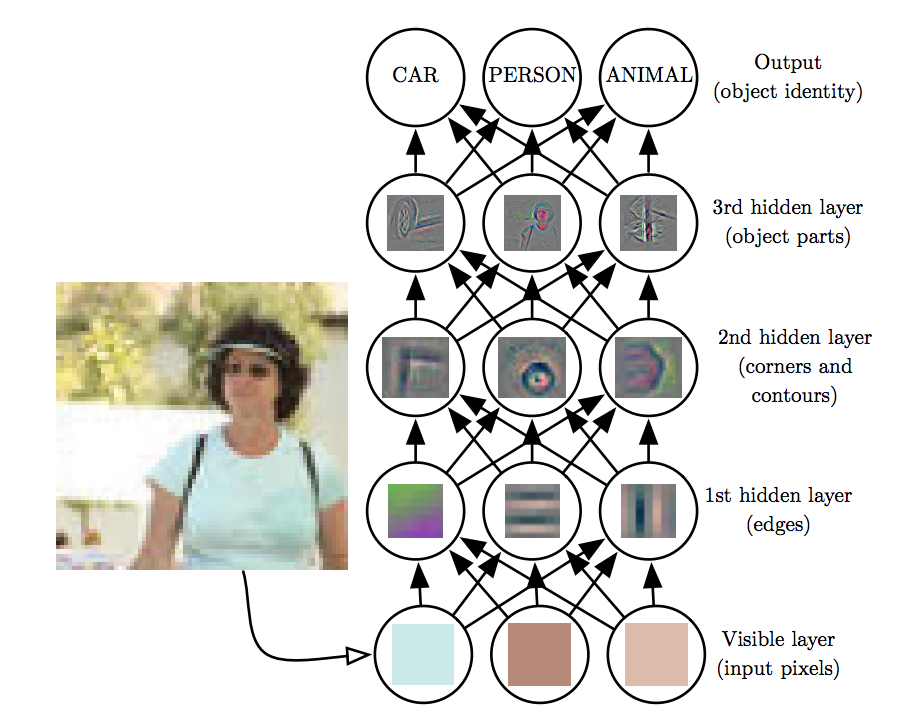
Deep Learning and Hierarchical Feature Learning 深度学习和分层特征学习

Deep learning leverages multiple layers to learn hierarchical representations: 深度学习利用多层来学习分层表示：

• Lower Layers: Capture simple features like edges or textures. 底层：捕捉简单特征，如边缘或纹理。
• Middle Layers: Combine simple features to form more complex patterns. 中间层：将简单特征组合成更复杂的模式。
• Higher Layers: Abstract high-level concepts relevant to the task. Higher Layers: 与任务相关的抽象高层概念。

This hierarchy enables neural networks to automatically learn features from raw data. 这种层次结构使神经网络能够自动从原始数据中学习特征。

Deep Learning and Hierarchical Feature Learning 深度学习和分层特征学习

Deep learning leverages multiple layers to learn hierarchical representations: 深度学习利用多层来学习分层表示：

• Lower Layers: Capture simple features like edges or textures. 底层：捕捉简单特征，如边缘或纹理。
• Middle Layers: Combine simple features to form more complex patterns. 中间层：将简单特征组合成更复杂的模式。
• Higher Layers: Abstract high-level concepts relevant to the task. Higher Layers: 与任务相关的抽象高层概念。

This hierarchy enables neural networks to automatically learn features from raw data. 这种层次结构使神经网络能够自动从原始数据中学习特征。

Feedforward step

To calculate the output of the $j$-th unit for the $i$-th data example we calculate

\[{o_j^{(i)}=\phi(z_j^{(i)});,\quad z_j^{(i)}=w_{0j}+\sum_{k=1}^{n_i}w_{kj}\cdot x_k^{(i)}}\]

If we have a $n_i$ input nodes and $n_0$ output units we have $(n_i +1)\times n_0$ parameters $w_{kj}$. We can organise them in a $n_i+1$ by $n_0$ matrix of parameters $W$ and write the vector of $x$ values for the $n_0$ output units as

\[z = W^Tx\]

where xx is the column vector of input values with a $1$ added as the $0$-th component.

The value $z$ is then passed through the non-linear function.

Last step

If we have more that 2 classes we want the last layer’s output to be probabilities of belonging to one the the $k$ classes in the classifier. For this we replace the sigmoid function with the softmax function:

\[{s_{i}(z)=\frac{e^{z_{i}}}{\Sigma_{j=1}^{k}e^{z_{j}}}}\]

It is by definition normalised such that the sum adds to one and is the multi-class generalisation of the sigmoid function. $s_i$ is largest for the index $i$ with the largest $z_i$. The classifier prediction will typically be the class $i$ with the largest value $s_i$.

\[\frac{\partial s_i}{\partial z_{j}}=\frac{-e^{z_{i}}e^{z_j}+\delta_{ij}e^{z_{i}}\Sigma_{i=1}^ke^{z_i}}{\left(\Sigma_{j=1}^ke^{z_j}\right)^{2}}={s}\frac{-e^{z_j}+\delta_{ij}\Sigma_{i=1}^{\mathrm{k}}e^{z_i}}{\Sigma_{j=1}^{k}e^{z_j}}={s}\left(\delta_{ij}-s_j\right)\]

Multi-class loss function

The generalistaion of the cross entropy loss for multiple class is given by

\[{J=-\sum_{i,j}y_{j}^{(i)}log(\hat y_{j}^{(i)})}\]

where $y^{(i)}_j$ is $1$ if training sample ii is in class $j$, 0 otherwise.

This is called one-hot encoding. The derivative of the loss function with respect to one of the predictions is given by

\[\frac{\partial J}{\partial \hat y_j^{(i)}}=-\frac{y_j^{(i)}}{\hat y_j^{(i)}}\]

Example

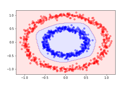
Using the same circle dataset that we used before, the decision function for a single-layer neural network with 10 hidden units gives the following decision boundary:

• Using a neural network to classify points in a circular pattern: 使用神经网络来对圆形模式中的点进行分类：
  • Data is not linearly separable. 数据不是线性可分的。
  • Single-layer networks fail to classify correctly. 单层网络无法正确分类。
  • Multi-layer networks with hidden units can capture the circular pattern. 具有隐藏单元的多层网络可以捕捉到循环模式。

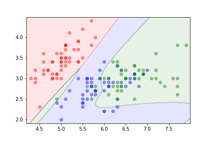
Here is an example using more than two classes.

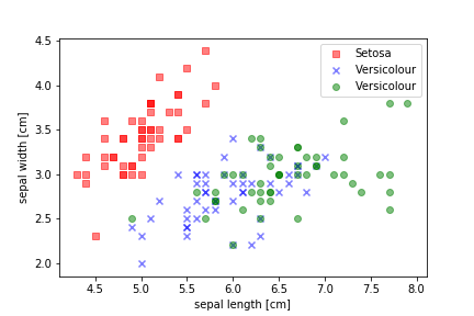
Iris Dataset 鸢尾花数据集

Classifying iris flowers into three species using a neural network: 将鸢尾花分为三个物种，使用神经网络：

• Features: sepal length, sepal width, petal length, petal width. 特征：萼片长度，萼片宽度，花瓣长度，花瓣宽度。
• Three classes: Setosa, Versicolor, Virginica. 三个类别：Setosa，Versicolor，Virginica。
• Multi-class classification using softmax output layer. 多类分类使用 softmax 输出层。

Training Neural Networks 训练神经网络

Training involves adjusting weights to minimize a loss function: 训练涉及调整权重以最小化损失函数：

1. Initialize weights randomly or using specific initialization methods. 随机初始化权重或使用特定的初始化方法。
2. Perform a forward pass to compute the output. 执行前向传播以计算输出。
3. Calculate the loss using a suitable loss function. 使用合适的损失函数计算损失。
4. Compute gradients via backpropagation. 通过反向传播计算梯度。
5. Update weights using an optimization algorithm. 使用优化算法更新权重。
6. Repeat the process for multiple epochs. 重复该过程多个时代。

Key concepts: 关键概念:

• Epoch: One complete pass through the training dataset. Epoch: 一次完整的训练数据集遍历。
• Batch Size: Number of samples processed before updating weights. 批量大小：在更新权重之前处理的样本数量。
• Learning Rate: Controls the step size during weight updates. 学习率：控制权重更新过程中的步长。

Weight Initialization Techniques 权重初始化技术

Proper weight initialization can help in faster convergence: 适当的权重初始化可以帮助加快收敛速度

• Zero Initialization: Not recommended as it causes symmetry. 零初始化：不建议，因为会导致对称性。
• Random Initialization: Small random values from a normal or uniform distribution. 随机初始化：从正态分布或均匀分布中取小的随机值。
• Xavier Initialization: Scales weights based on the number of input and output neurons. Xavier 初始化：根据输入和输出神经元的数量来缩放权重。
• He Initialization: Similar to Xavier but designed for ReLU activation functions. He 初始化：类似于 Xavier，但设计用于 ReLU 激活函数。

Avoiding vanishing or exploding gradients through appropriate initialization. 避免通过适当的初始化消失或爆炸的梯度。

Feedforward Process 前馈过程

The feedforward process involves propagating inputs through the network to generate an output. 前馈过程涉及通过网络传播输入以生成输出。

1. Input data is presented to the input layer. 输入数据被呈现到输入层。
2. Each neuron computes a weighted sum of its inputs and applies an activation function. 每个神经元计算其输入的加权和并应用激活函数。
3. The outputs of one layer become the inputs to the next layer. 一个图层的输出成为下一层的输入。
4. The final output layer produces the network’s prediction. 最终输出层产生网络的预测。

This process is used during both training and inference phases. 这个过程在训练和推断阶段都会使用。

Feedforward Process 前馈过程

Activation Functions 激活函数

Activation functions introduce non-linearity into the neural network, allowing it to learn complex patterns. 激活函数引入非线性到神经网络中，使其能够学习复杂模式。

Common activation functions include: 常见的激活函数包括：

• Step Function
• Sigmoid Function Sigmoid 函数
• Tanh Function 双曲正切函数
• ReLU (Rectified Linear Unit) ReLU (修正线性单元)
• Leaky ReLU
• ELU (Exponential Linear Unit) ELU (指数线性单元)
• Softmax Function Softmax 函数

Selection of activation functions can significantly impact the network’s performance. 激活函数的选择可以显著影响网络的性能。

Activation Functions 激活函数

1. Step Function

   • Formula \(\phi(x)=\left\{\begin{array}{cc}1&\mathrm{if~}x\geq0\\0&\mathrm{if~}x<0\end{array}\right.\)

   • Characteristics

     特征:

     • Binary output (0 or 1). 二进制输出（0 或 1）。
     • Non-differentiable at $x=0$.
     • Historically used in perceptrons but less common in modern networks. 在感知器中历史上使用过，但在现代网络中不太常见。

Sigmoid Function Sigmoid 函数

• Formula \(\phi(x)=\frac1{1+e^{-x}}\)

• Characteristics

  特征:

  • Output ranges between 0 and 1. 输出范围在 0 和 1 之间。
  • Smooth and differentiable. 平滑且可微。
  • Can cause vanishing gradient problems in deep networks. 可以在深度网络中引起梯度消失问题。

• Tanh Function 双曲正切函数

• Formula \(\phi(x)=\tanh(x)=\frac{e^x-e^{-x}}{e^x+e^{-x}}\)

• Characteristics

  特征:

  • Output ranges between -1 and 1. 输出范围在-1 和 1 之间。
  • Zero-centered, which can be advantageous. 零中心化，这可能是有利的。
  • Also susceptible to vanishing gradients. 也容易受到消失梯度的影响。

ReLU (Rectified Linear Unit) ReLU (修正线性单元)

• Formula \(\phi(x) = max(0,x)\)

• Characteristics

  特征:

  • Outputs zero for negative inputs and linear for positive inputs. 对负输入输出零，对正输入输出线性。
  • Simple and computationally efficient. 简单且计算效率高。
  • Helps mitigate vanishing gradient problems. 帮助缓解梯度消失问题。
  • Can suffer from “dying ReLUs” where neurons stop activating. 可以遭受“死亡 ReLUs” 的问题，即神经元停止激活。

• Leaky ReLU

• Formula \(\phi(x)=\left\{\begin{array}{ll}x&\mathrm{if~}x\geq0\\\alpha x&\mathrm{if~}x<0\end{array}\right.\) Typically, $\alpha$ is a small constant like 0.01. 通常， $\alpha$​是一个小常数，比如 0.01。

• Characteristics

  特征:

  • Allows a small, non-zero gradient when$ x<0$. 允许在 $ x<0$ 时存在微小的非零梯度。
  • Addresses the “dying ReLU” problem. 解决“濒死的 ReLU”问题。

Softmax Function Softmax 函数

• Formula \(\phi(x_i)=\frac{e^{x_i}}{\sum_je^{x_j}}\)

• Characteristics

  特征:

  • Converts logits into probabilities that sum to 1. 将对数几率转换为总和为 1 的概率。
  • Commonly used in the output layer for multi-class classification. 常用于多类分类的输出层。

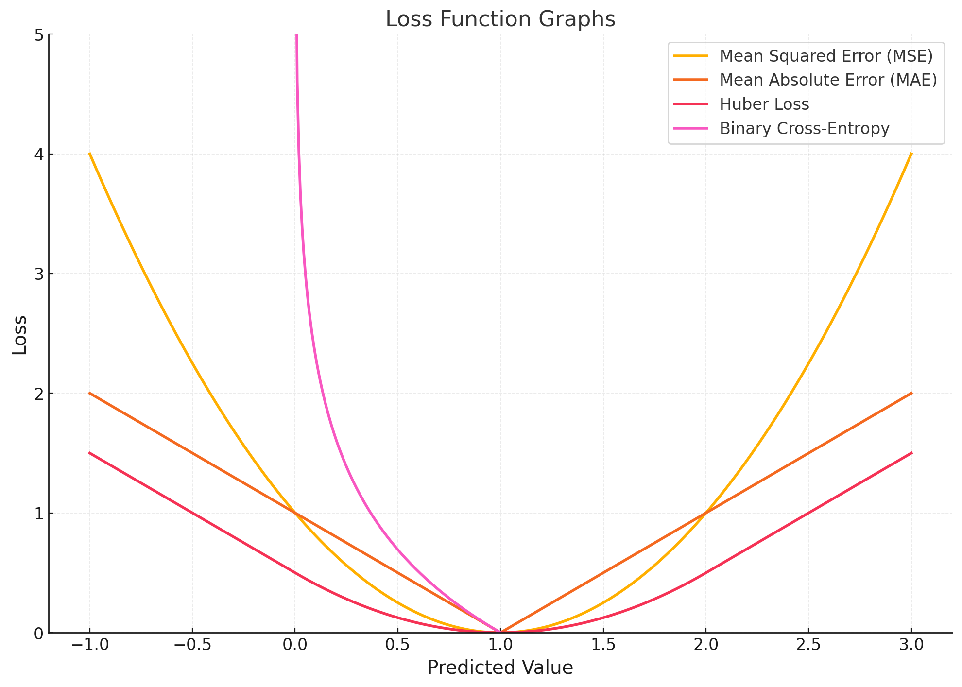
Loss Functions 损失函数

Loss functions quantify the difference between the predicted output of the network and the true output. They are crucial for training neural networks using backpropagation. 损失函数量化了网络预测输出与真实输出之间的差异。它们对使用反向传播训练神经网络至关重要。

Common loss functions include: 常见的损失函数包括：

• Mean Squared Error (MSE) 均方误差（MSE）
• Mean Absolute Error (MAE) 平均绝对误差（MAE）
• Binary Cross-Entropy Loss (Log Loss) 二元交叉熵损失（对数损失）
• Categorical Cross-Entropy Loss 分类交叉熵损失
• Hinge Loss
• Kullback-Leibler Divergence Loss (KL Divergence)

1. Mean Squared Error (MSE) 均方误差（MSE）

   • Formula \(L_}=\frac{1}{n}\sum_{i=1}^{n}(y_{i}-\hat{y}_{i})^{2}\)

   • Explanation

     • $y_i$: True value. 真实值。
     • $\hat y_i$: Predicted value. 预测值。
     • Measures the average squared difference between predictions and actual values. 衡量预测值与实际值之间的平均平方差。

   • Usage

     使用：

     • Commonly used in regression problems. 常用于回归问题。
     • Penalizes larger errors more than smaller ones. 惩罚较大的错误比较小的错误更多。

Mean Absolute Error (MAE) 平均绝对误差（MAE）

• Formula \(L_}=\frac{1}{n}\sum_{i=1}^{n}|y_{i}-\hat{y}_{i}|\)

• Explanation

  • Measures the average absolute difference between predictions and actual values. 衡量预测值与实际值之间的平均绝对差异。

• Usage

  使用：

  • Used in regression problems where outliers are less significant. 用于回归问题中，异常值影响较小。
  • Less sensitive to outliers compared to MSE. 相对于均方误差（MSE），对异常值不太敏感。

Binary Cross-Entropy Loss (Log Loss) 二元交叉熵损失（对数损失）

• Formula \(L_{\mathrm{Binary}}=-\frac1n\sum_{i=1}^n[y_i\log(\hat{y}_i)+(1-y_i)\log(1-\hat{y}_i)]\)

• Explanation

  • Used for binary classification tasks. 用于二元分类任务。
  • Penalizes the divergence between predicted probabilities and actual labels. 惩罚预测概率与实际标签之间的差异。

• Usage

  使用：

  • Applicable when outputs are probabilities (using sigmoid activation in the output layer). 适用于输出为概率时（在输出层使用 sigmoid 激活）。

Categorical Cross-Entropy Loss 分类交叉熵损失

• Formula \(L_{\text{Categorical}}=-\sum_{i=1}^{n}\sum_{k=1}^{K}y_{i,k}\log(\hat{y}_{i,k})\)

• Explanation

  • $y_{i,k}$: Binary indicator (0 or 1) if class label $k$ is the correct classification for sample $i$.
  • $\hat y_{i,k}$: Predicted probability that sample $i$ is of class $k$. 预测样本 $i$ 属于类别 $k$ 的概率。
  • Used for multi-class classification tasks. 用于多类分类任务。

• Usage

  使用：

  • Often used with softmax activation in the output layer. 通常与输出层中的 softmax 激活一起使用。

Hinge Loss

• Formula \(L_}=\frac{1}{n}\sum_{i=1}^{n}\max(0,1-y_{i}\hat{y}_{i})\)

• Explanation

  • Used primarily for “maximum-margin” classification, especially with support vector machines. 主要用于“最大间隔”分类，特别是支持向量机。
  • yiyi should be -1 or 1, representing class labels. yiyi 应该是 -1 或 1，代表类别标签。

• Usage

  使用：

  • Can be used in neural networks for binary classification. 可以用于神经网络进行二元分类。

Kullback-Leibler Divergence Loss (KL Divergence)

• Formula \(L_}=\sum_{i=1}^{n}y_{i}\log\left(\frac{y_{i}}{\hat{y}_{i}}\right)\)

• Explanation

  • Measures how one probability distribution diverges from a second, expected probability distribution. 衡量一个概率分布与第二个预期概率分布的差异。

• Usage

  使用：

  • Used in applications like variational autoencoders. 用于诸如变分自动编码器之类的应用。

Role in Backpropagation: 反向传播中的角色:

• The loss function calculates the error between the network’s predictions and the true values. 损失函数计算网络预测值与真实值之间的误差。
• The computed loss is then used to calculate gradients during backpropagation. 计算得到的损失然后用于在反向传播过程中计算梯度。
• The gradients are propagated backward through the network to update the weights. 梯度通过网络向后传播以更新权重。

Understanding and selecting the appropriate loss function is critical for effective training of neural networks. 了解和选择适当的损失函数对于有效训练神经网络至关重要。

Compute gradients via backpropagation. 通过反向传播计算梯度。

Backpropagation 反向传播

Backpropagation is the algorithm used to train neural networks: 反向传播是用于训练神经网络的算法

1. Computes the gradient of the loss function with respect to each weight by the chain rule. 计算损失函数相对于每个权重的梯度，使用链式法则。
2. Updates weights in the opposite direction of the gradient. 沿着梯度的相反方向更新权重。
3. Repeats the process for multiple iterations (epochs). 重复该过程多次迭代（时期）。

Gradient Descent 梯度下降

Gradient descent is the optimization algorithm used to minimize the loss function. 梯度下降是用于最小化损失函数的优化算法。

Update rule: 更新规则: \(w_{ij}=w_{ij}-\eta\frac{\partial J}{\partial w_{ij}}\) where: 在哪里:

• $\eta$ = learning rate.
• $\frac{\partial J}{\partial w_{ij}}$ = gradient of the loss with respect to weight wijwij.

Variants: 变体:

• Batch Gradient Descent 批量梯度下降
• Stochastic Gradient Descent (SGD) 随机梯度下降（SGD）
• Mini-Batch Gradient Descent 小批量梯度下降

Optimization Algorithms 优化算法

Various optimization algorithms improve training efficiency and convergence: 各种优化算法提高训练效率和收敛性：

• Stochastic Gradient Descent (SGD): Updates weights using individual samples. 随机梯度下降（SGD）：使用单个样本更新权重。
• Momentum: Accelerates SGD by considering past gradients. 动量：通过考虑过去的梯度来加速 SGD。
• Adagrad: Adapts learning rate based on past gradients. Adagrad: 根据过去的梯度调整学习率。

Choice of optimizer can significantly affect training performance. 优化器的选择可以显著影响训练性能。

1. Stochastic Gradient Descent (SGD) 随机梯度下降（SGD）

   • Update Rule \(w_{t+1}=w_t-\eta\nabla L(w_t;x_i,y_i)\)

   • Explanation

     • Updates weights using individual samples $(x_i,y_i)$. 使用单个样本 更新权重。
     • $\eta$ is the learning rate. 是学习率。
     • $ \nabla L(w_t;x_i,y_i)$ is the gradient of the loss function at time t. 是时间 t 的损失函数的梯度。

   • Characteristics

     特征:

     • Introduces noise due to sampling, which can help escape local minima. 引入由采样引起的噪声，有助于逃离局部最小值。
     • Can be slow to converge near minima. 可能会在极小值附近收敛较慢。

Momentum 动量

• Update Rule \(\begin{aligned}v_t&=\gamma v_{t-1}+\eta\nabla L(w_t)\\w_{t+1}&=w_t-v_t\end{aligned}\)

• Explanation

  • $v_t$ is the velocity (accumulated gradient). 是速度（累积梯度）。
  • $\gamma$ is the momentum coefficient (typically between 0 and 1).
  • Accelerates SGD by smoothing gradients over time. 通过随时间平滑梯度来加速 SGD。

• Characteristics

  特征:

  • Helps navigate ravines in the loss surface. 帮助在损失表面中导航峡谷。
  • Can overshoot minima if $\gamma$ is too high.

Adagrad

• Update Rule

  \[\begin{aligned} G_{t}& =G_{t-1}+\nabla L(w_t)^2 \\ w_{t+1}& =w_t-\frac\eta{\sqrt{G_t+\epsilon}}\nabla L(w_t) \end{aligned}\]

• Explanation

  • $G_t$ is the sum of the squares of past gradients (element-wise). 是过去梯度平方的总和（逐元素）。
  • $\epsilon$ is a small constant to prevent division by zero (e.g., $10^{-8}$). 是一个小常数，用于防止除以零
  • Adapts the learning rate for each parameter individually. 为每个参数单独调整学习率。

• Characteristics

  特征:

  • Good for sparse data. 适用于稀疏数据。
  • Learning rate diminishes over time, which can halt training prematurely. 学习速率随时间减小，这可能会导致训练过早停止。

Challenges in Training Deep Networks 训练深度网络中的挑战

Deep networks introduce specific challenges: 深度网络引入了特定的挑战：

• Vanishing Gradients: Gradients become very small, slowing down learning. 梯度消失：梯度变得非常小，减慢学习速度。
• Exploding Gradients: Gradients grow exponentially, causing instability. 梯度爆炸：梯度呈指数增长，导致不稳定。
• Overfitting: Model performs well on training data but poorly on unseen data. 过拟合：模型在训练数据上表现良好，但在未见数据上表现不佳。
• Computational Complexity: Increased number of parameters requires more computational resources. 计算复杂性：增加参数数量需要更多的计算资源。

Strategies to mitigate these issues include activation function choices, gradient clipping, and regularization. 缓解这些问题的策略包括激活函数选择、梯度裁剪和正则化。

Batch Normalization 批量归一化

Batch normalization is a technique to improve training speed and stability: 批量归一化是一种提高训练速度和稳定性的技术

• Normalizes the input of each layer to have zero mean and unit variance. 将每一层的输入标准化为零均值和单位方差。
• Reduces internal covariate shift. 减少内部协变量转移。
• Allows for higher learning rates. 允许更高的学习速率。
• Acts as a form of regularization. 作为一种规范化形式。

Regularization Techniques 正则化技术

To prevent overfitting, we use regularization methods: 为了防止过拟合，我们使用正则化方法：

• L1 and L2 Regularization: Add penalty terms to the loss function. L1 和 L2 正则化：向损失函数添加惩罚项。
• Dropout: Randomly drop units during training to prevent co-adaptation. 辍学：在训练过程中随机丢弃单元以防止共适应。
• Early Stopping: Stop training when validation loss starts to increase. 早停止：当验证损失开始增加时停止训练。
• Data Augmentation: Increase the size of the training data by transformations. 数据增强：通过转换增加训练数据的大小。
• Ensemble Methods: Combine multiple models to improve generalization. 集成方法：结合多个模型以提高泛化能力。

Regularization helps in building models that generalize well to new data. 正则化有助于构建能够很好泛化到新数据的模型。

Practical Considerations 实际考虑

Important aspects to consider when working with neural networks: 使用神经网络时需要考虑的重要方面：

• Hyperparameter Tuning: Selecting learning rates, batch sizes, number of layers, etc. 超参数调整：选择学习率、批量大小、层数等。
• Data Preprocessing: Normalization, scaling, and handling missing data. 数据预处理：标准化、缩放和处理缺失数据。
• Hardware Acceleration: Utilizing GPUs and TPUs for faster computation. 硬件加速：利用 GPU 和 TPU 进行更快的计算。
• Frameworks and Libraries: TensorFlow, PyTorch, Keras, etc. 框架和库：TensorFlow，PyTorch，Keras 等。
• Model Interpretability: Understanding and explaining model decisions. 模型可解释性：理解和解释模型决策。

These factors can significantly impact the performance and usability of neural network models. 这些因素可以显著影响神经网络模型的性能和可用性。

Network Architectures 网络架构

Neural networks are constructed by connecting artificial neurons in various configurations. 神经网络是通过连接不同配置的人工神经元构建的。

Types of network architectures: 网络架构类型:

• Feedforward Neural Networks: Information moves only in one direction, from input to output. 前馈神经网络：信息只能沿一个方向传递，从输入到输出。
• Convolutional Neural Networks (CNNs): Specialized for processing grid-like data such as images. 卷积神经网络（CNNs）：专门用于处理像图像这样的网格数据。
• Recurrent Neural Networks (RNNs): Designed for sequential data, with loops to allow information to persist. 递归神经网络（RNNs）：设计用于序列数据，具有循环以允许信息持续存在。
• Autoencoders: Used for unsupervised learning of efficient codings. 自动编码器：用于无监督学习高效编码。
• Generative Adversarial Networks (GANs): Consist of generator and discriminator networks for data generation. 生成对抗网络（GANs）：由生成器和判别器网络组成，用于数据生成。
• Transformer Networks: Utilize self-attention mechanisms, prominent in NLP tasks. Transformer Networks: 利用在自然语言处理任务中突出的自注意力机制。

Each architecture is tailored for specific types of data and tasks. 每种架构都针对特定类型的数据和任务进行了定制。

Advanced Topics in Deep Learning 深度学习的高级主题

Exploring cutting-edge developments in deep learning: 探索深度学习的前沿发展：

• Attention Mechanisms: Allow models to focus on specific parts of the input. 注意机制：允许模型专注于输入的特定部分。
• Transfer Learning: Leveraging pre-trained models for new tasks. 迁移学习：利用预训练模型进行新任务。
• Generative Models: GANs and Variational Autoencoders (VAEs). 生成模型：GAN 和变分自动编码器（VAEs）。
• Self-Supervised Learning: Learning representations from unlabeled data. 自监督学习：从无标签数据中学习表示。
• Reinforcement Learning: Training agents to make decisions through rewards. 强化学习：通过奖励训练代理程序做出决策。

These topics represent the forefront of research and applications in deep learning. 这些主题代表了深度学习领域的研究和应用的前沿。