IML L7.2 Principal component analysis

Principal component analysis

If we have many features, odds are that many are correlated. If there are strong relationships between features, we might not need all of them.

With principal component analysis we want to extract the most relevant/independant combination of features.

It is important to realise that PCA only looks at the features without looking at the labels, it is an example of unsupervised learning.

Correlated vs uncorrelated

Correlated features

Uncorrelated features:

The idea for PCA is to project the data on a subspace with fewer dimensions.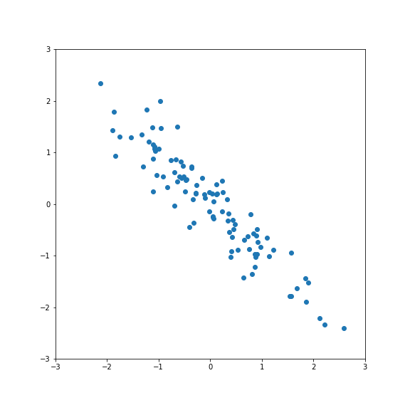

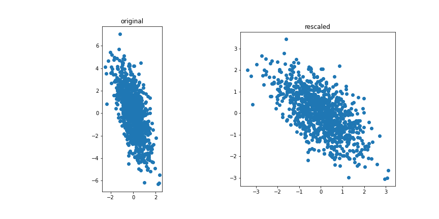
The data is standardised.

If we project onto the first component we get variance 1: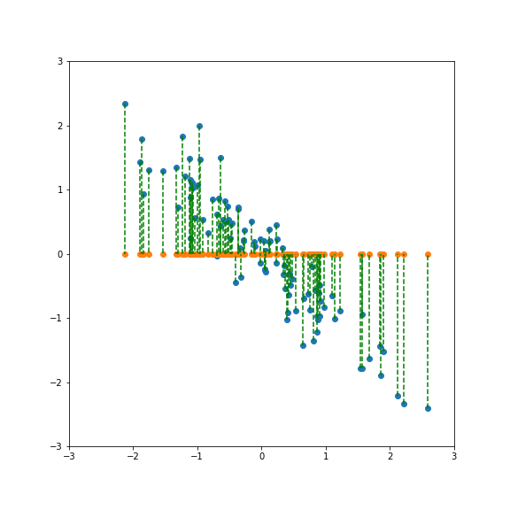

If we project onto the second component we also get variance 1: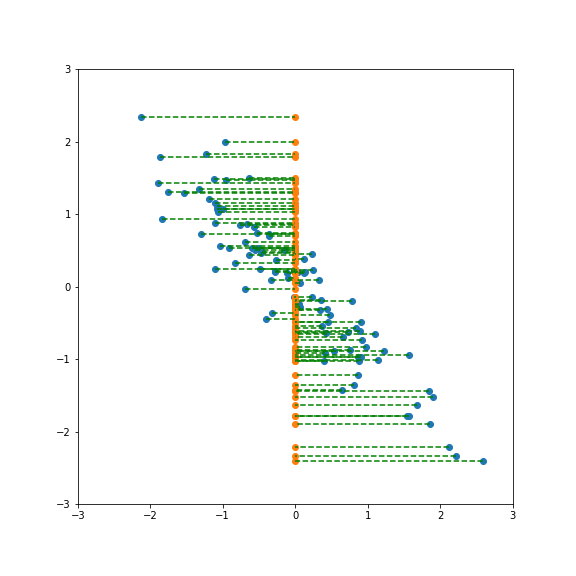

But projecting onto a different direction gives a different variance, here larger than 1: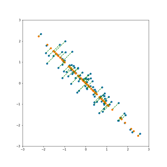

And here smaller than one: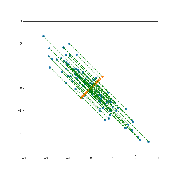

Performing PCA gives a new basis in feature space that include the direction of largest and smallest variance.

There is no guarantee that the most relevant features for a given classification tasks are going to have the largest variance.

If there is a strong linear relationship between features it will correspond to a component with a small variance, so dropping it will not lead to a large loss of variance but will reduce the dimensionality of the model.

Finding the principal components

The first step is to normalise and center the features.

xi→axi+bxi→axi+b

such that

⟨xi⟩=0,⟨x2i⟩=1⟨xi⟩=0,⟨xi2⟩=1

The covariance matrix of the data is then given by

σ=XTXσ=XTX

If XX is the nd×nfnd×nf data matrix of the ndnd training samples with nfnf features. The covariance matrix is a nf×nfnf×nf matrix.

If we diagonalize σσ

σ=SDS−1σ=SDS−1

where the columns of SS are the eigenvectors of σσ.

the eigenvectors with the highest eigenvalues correspond to the axis with the highest variance. PCA reduces the dimensionality of the data by projecting unto the subspace spanned by the eignevectors with the kk highest eigenvalues.

Xk=XSkXk=XSk

where SkSk is the nf×knf×k matrix composed of the kk highest eigenvectors.

Singular value decomposition

There is a shortcut to computing the full data variance to calculate the principal component analysis. Using singular value decomposition, we can write XX as

X=UΣVX=UΣV

where UU is an orthogonal nd×ndnd×nd matrix, ΣΣ is a nd×nfnd×nf matrix with non-vanishing elements only on the diagonal and VV is a nf×nfnf×nf orthogonal matrix.

using this decomposition we have

XTX=VTΣTUTUΣV=V−1ΣTΣVXTX=VTΣTUTUΣV=V−1ΣTΣV

The combination ΣTΣΣTΣ is diagonal so we see that the matrix V is the change of basis needed to diagonalise XTXXTX. So we only need to perform the SVD of X to find the eigenvectors of XTXXTX.

Data sample variance

The total variance of a data (zero-centered) sample is given by

σtot=⟨∑iX2i⟩=1N−1∑sample∑ix2i=1N−1Tr(XTX).σtot=⟨∑iXi2⟩=1N−1∑sample∑ixi2=1N−1Tr(XTX).

The trace is invariant under rotations in the feature space so it is equal to the trace of the diagonalised matrix Tr(σ)=∑EjTr(σ)=∑Ej where EjEj are the eigenvalues of XTXXTX.

If we have the SVD decomposition of XX we can express these eigenvalues in term of the diagonal elements ϵjϵj of ΣΣ:

Tr(σ)=∑Ej=∑jϵ2j

Explained variance

When we only consider the kk principal axis of a dataset we will loose some of the variance of the dataset.

Assuming the eigenvalues are ordered in size we have

σk≡Tr(XTkXk)=k∑j=1ϵ2jσk≡Tr(XkTXk)=∑j=1kϵj2

σkσk is the variance our reduced dataset retained from the original, it is often referred as the explained variance.

Example: 8x8 digits pictures

We consider a dataset of handwritten digits, compressed to an 8x8 image:

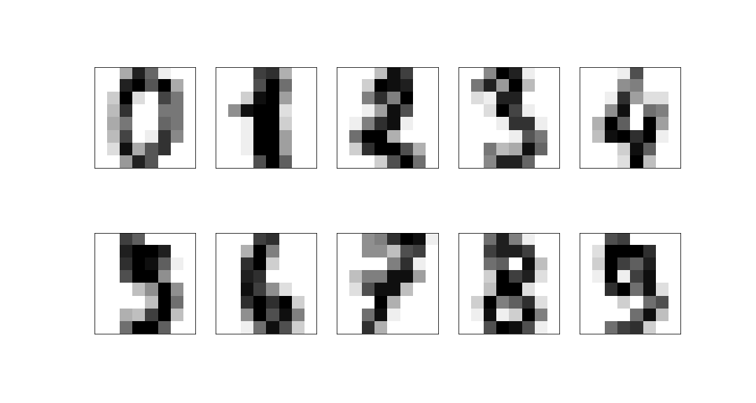
These have a 64-dimensional space but this is clearly far larger than the true dimension of the space:

• only a very limited subset of 8x8 pictures represent digits
• the corners are largely irrelevant hardly ever used
• digits are lines, so there is a large correlation between neighbouring pixels.

PCA should help us limit our features to things that are likely to be relevant.

Performing PCA we can see how many eigenvectors are needed to reproduce a given fraction of the dataset variance:

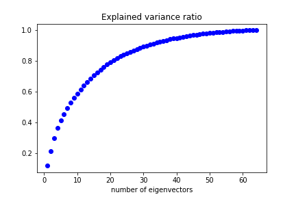
We can keep 50% of the dataset variance with less than 10 features.

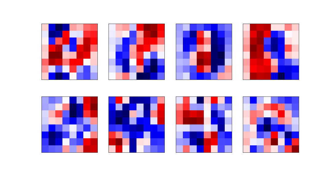
he eight most relevant eigenvectors are:

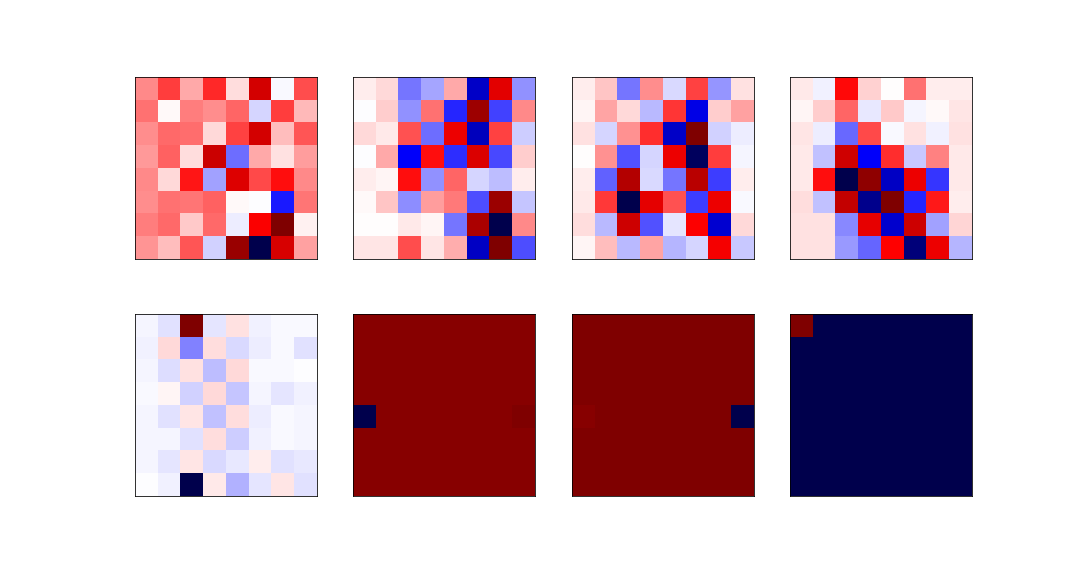
The least relevant eigenvectors are:

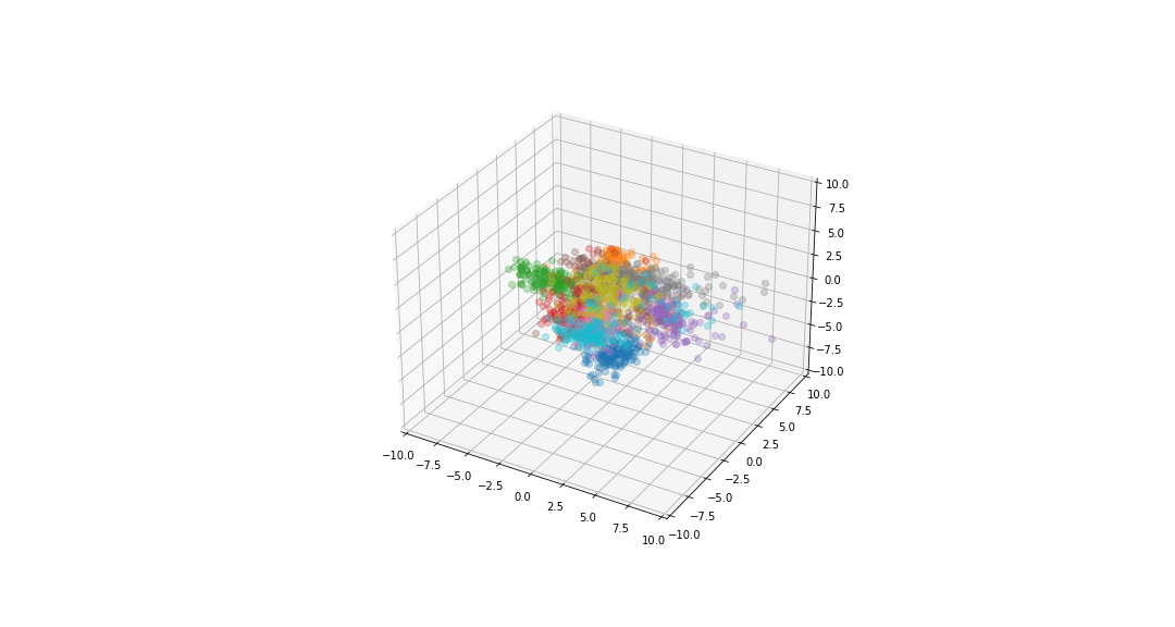
Data visualisation

If we reduce the data to be 2-dimensional or 3-dimensional we can get a visualisation of the data.

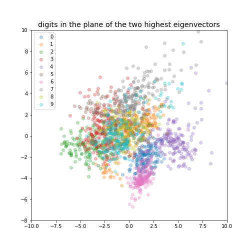
digits in the plane of the two highest eigenvectors