IML L8.1 Using scikit-learn
Using scikit-learn
scikit-learn and pandas are the common tools for data science in python.
1
2
3
import sklearn
import numpy as np
import matplotlib.pyplot as plt
Scikit-learn
sklearn has many of the tools needed to set up a data analysis pipeline:
- preprocessors
- models
- model selection
Preprocessor
Preprocessors include
standardScaler: shifts and scale the data to have mean 0 and standard deviation 1.Normalizer: normalises the features for each data sample to have unit lenghtMinMaxScaler: shifts and scales the data so it fits in a given intervalOneHotEncoder: transforms class labels to a one-hot encoded matrix of 0 or 1 valuesPolynomialFeatures: Creates polynomial features- …
Models
in sklearn.linear_model:
LogisticRegression: the logistic regression classifier discussed in Lecture 2.Ridge: the ridge regression discussed in Lecture 4Perceptron: the perceptron model discussed in Lecture 1
in sklearn.neural_network:
MLPclassifier: the multiple layer perceptron ‘classic’ neural network discussed in lecture 5 and 6.
in sklearn.neighbors:
KNeighborsClassifier: the kk-neighbours classifier discussed in Lecture 7.
in sklearn.svm:
SVC: the support vector classifier discussed in Lecture 3.
Interface
The preprocessors and models in sklearn have a common functions:
fit: fits to the data to set the model/preprocessor parameterstransform(): transforms the input data and returns the transformed datafit_transform(): do both operations
Models have common functions:
predict(X): make a prediction for new dataXscore(X,y): gives the score for dataXand targetsy
fit example
1
2
3
4
from sklearn.preprocessing import StandardScaler
stdScaler = StandardScaler()
randomData = np.random.normal(2,3,size=(1000,1) )
stdScaler.fit(randomData)
StandardScaler()
After the fit the standard scaler has leaned the mean and standard deviation of the dataset
1
stdScaler.mean_, stdScaler.scale_
Out[3]:
1
(array([1.9907856]), array([2.92175702]))
It can now apply the same transformation to unseen data:
In [4]:
1
2
3
4
5
stdScaler.transform([
    [2],
    [5],
    [-1]
])
Out[4]:
1
2
3
array([[ 0.00315372],
       [ 1.02993315],
       [-1.02362571]])
Tools
in model_selection:
learning_curve: can be used to produce learning curves.train_test_split: can be used to separate a given dataset in a training and validation sample.GridSearchCV: can be used to scan through a grid of parameter through cross validation.
Model selection with GridSearchCV
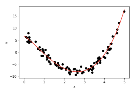
We start with the same dataset as in one of the exercises:
1
2
3
4
5
6
7
8
9
def fn(x):
    return 7 - 8*x - 0.5*x**2 + 0.5*x**3

n_train = 100
np.random.seed(1122)
xs = np.linspace(0, 5)
rxs = 5 * np.random.random(n_train)
X1D = np.array([rxs]).T
ys1D = fn(rxs) + np.random.normal(size = (n_train) )
1
2
3
4
5
plt.plot(xs, fn(xs), 'b--')
plt.plot(rxs, ys1D, 'ok')
plt.xlabel('x');
plt.ylabel('y');

1
2
3
4
5
6
7
8
9
10
11
12
from sklearn.model_selection import GridSearchCV
from sklearn.linear_model import Ridge
from sklearn.preprocessing import PolynomialFeatures

polynomial_features = PolynomialFeatures(degree=8)
X_train = polynomial_features.fit_transform(X1D)

alpha_values = np.logspace(-4, 4, 100)
parameters = {'alpha': alpha_values}
r = Ridge()
Rsearch = GridSearchCV(r, parameters, cv=5)
Rsearch.fit(X_train, ys1D);
Our grid search has trained a ridge regression for each values of αα and performed a 5-fold cross validation, so we will have access to an average and an uncertainty estimate.
1
Rsearch.cv_results_.keys()
1
dict_keys(['mean_fit_time', 'std_fit_time', 'mean_score_time', 'std_score_time', 'param_alpha', 'params', 'split0_test_score', 'split1_test_score', 'split2_test_score', 'split3_test_score', 'split4_test_score', 'mean_test_score', 'std_test_score', 'rank_test_score'])
We can now plot the score as a function of α:
1
2
3
4
5
6
7
8
scores = Rsearch.cv_results_['mean_test_score']
scores_std = Rsearch.cv_results_['std_test_score']
plt.fill_between(alpha_values, scores - scores_std,
                 scores + scores_std, alpha=0.1, color="g")
plt.plot(alpha_values, scores)
plt.xscale('log')
plt.xlabel(r'Regularisation parameter $\alpha$')
plt.ylabel('Average score');

We can access the best model using best_estimator_:
In [10]:
1
2
3
4
5
6
7
8
9
xval = np.arange(0,5.1,0.1).reshape(-1, 1)
pxval = polynomial_features.transform(xval)
ypred = Rsearch.best_estimator_.predict(pxval)

plt.plot(rxs, ys1D,'ok')
plt.plot(xval, ypred , color='r')

plt.xlabel('x')
plt.ylabel('y');

Pipelines
You noticed that we had to remember all the steps of the training to make the prediction of the model for the preceding plot. This is akward and error-prone.
We can use Pipeline to create all steps of an analysis in one object.
1
2
3
4
5
6
from sklearn.pipeline import Pipeline

analysis_pipeline = Pipeline([
    ('poly', PolynomialFeatures(degree=8)),
    ('ridge', Ridge())
])
This pipeline can be used as a normal model, for example we can use it in a grid search:
1
2
3
4
5
6
7
8
degrees = [5,6,7]
parameters = {
    'ridge__alpha': alpha_values,
    'poly__degree': degrees
}
Psearch = GridSearchCV(analysis_pipeline, parameters, cv=5)
Psearch.fit(X1D, ys1D);
Notice how parameters of specific steps can be set!
We can plot the scores for each polynomial order:
1
2
3
4
5
6
7
8
9
10
for j in range(3):
    scores = Psearch.cv_results_['mean_test_score'][j*100:(j+1)*100]
    scores_std = Psearch.cv_results_['std_test_score'][j*100:(j+1)*100]
    plt.fill_between(alpha_values, scores - scores_std,
                 scores + scores_std, alpha=0.1, label="n={}".format(degrees[j]))
    plt.plot(alpha_values, scores)
plt.xscale('log')
plt.legend()
plt.xlabel(r'Regularisation parameter $\alpha$')
plt.ylabel('Test score');

And plot the best estimator’s prediction:
1
2
3
4
5
6
7
8
xval = np.arange(0,5.1,0.1).reshape(-1, 1)
ypred = Psearch.best_estimator_.predict(xval)

plt.plot(rxs, ys1D,'ok')
plt.plot(xval, ypred , color='r')

plt.xlabel('x')
plt.ylabel('y');
Notice how we did not need to explicitely perform all the steps.
1
2
3
4
5
6
7
8
9
10
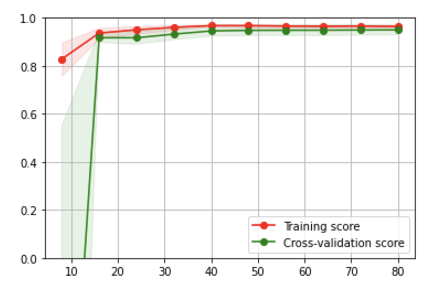
11
plt.fill_between(train_sizes, train_scores_mean - train_scores_std,
train_scores_mean + train_scores_std, alpha=0.1, color="r")
plt.fill_between(train_sizes, test_scores_mean - test_scores_std,
test_scores_mean + test_scores_std, alpha=0.1, color="g")
plt.plot(train_sizes, train_scores_mean, 'o-', color="r",
label="Training score")
plt.plot(train_sizes, test_scores_mean, 'o-', color="g",
label="Cross-validation score")
plt.ylim(0,1); plt.grid(); plt.legend(loc="best");