PO Lecture 5 Profiling

PO Lecture 5 Profiling

Large code bases

Performance counters

Unsuitable: too much code to annotate.
Which section(s) of the code takes most of the time?

Profiling to keep focus

1. Find hotspots (where most time is spent)
2. Measure performance of hotspots
3. Optimise hotspots

Profiling: types

Sampling

• ✔ Works with unmodified executables
• ❌ Only a statistical model of code execution
• ❌ Not very detailed for volatile metrics
• ❌ Needs long-running application

Instrumentation

• ✔ Maximally detailed and focused
• ❌ Requires annotations in source code
• ❌ Preprocessing of source required
• ❌ Can have large overheads for small functions.

Sampling

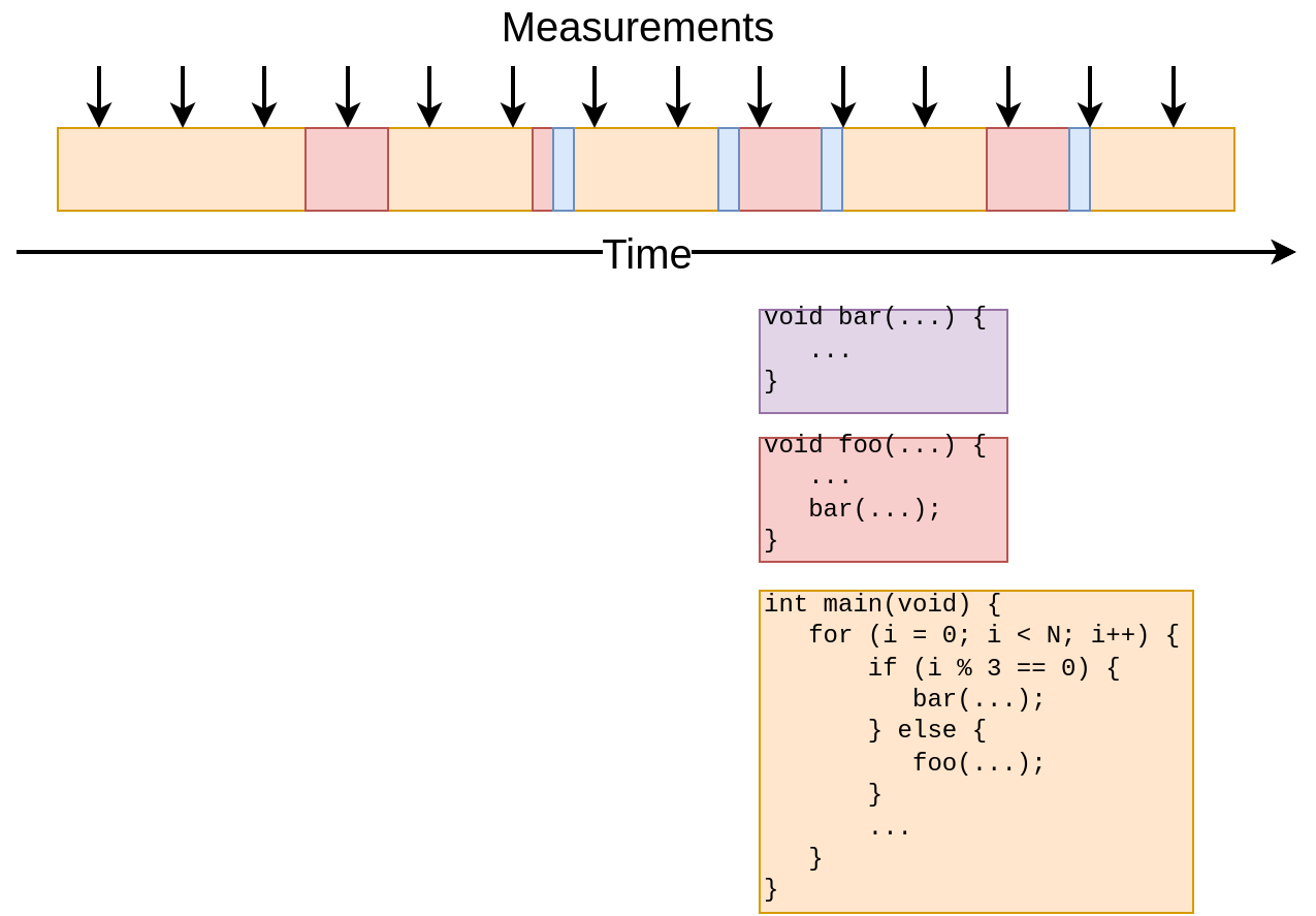
• Program interrupts
• Periodic measurements
• Snapshot of the stack
• Potentially inaccurate

void bar(...) {
    ...
}

void foo(...) {
    ...
    bar(...);
}

int main(void) {
    for (i = 0; i < N; i++) {
        if (i % 3 == 0) {
            bar(...);
        } else {
            foo(...);
        }
    }
    ...
}

Tracing

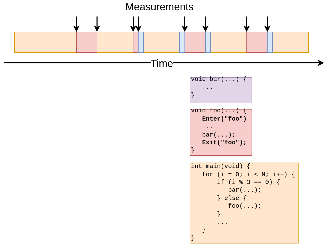
• Explicit measurement
• Extremely accurate
• Less information
• More work

Sampling profiles with gprof

Workflow

1. Compile with profiling information and debugging symbols
   gcc -pg -g <source_file> -o <executable_name>
2. Run code to produce file gmon.out
3. Generate output with
   gprof <executable_name> gmon.out # flat profile and
   # call graph
gprof -A <executable_name> gmon.out # annotated source

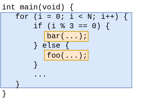
Instrumentation & sampling

• Code is instrumented by GCC
• Automatic tracing of all calls
• Triggering of measurement is sampling based (not every call)
• Trade-off approach

Output

• flat profile: time in function, number of function calls
• call graph: which function call which
• annotated source: number of time each line is executed

Output: the flat profile

Flat profile:

Each sample counts as 0.01 seconds.  
 % cumulative  self  self   total  
 time seconds   seconds calls  s/call name  
99.82  5.70      5.70   2     2.85   basic_gemm  
0.18   5.71      0.01   1     0.01   zero_matrix  
0.00   5.71      0.00   3     0.00   alloc_matrix  
0.00   5.71      0.00   3     0.00   free_matrix  
0.00   5.71      0.00   2     0.00   random_matrix  
0.00   5.71      0.00   1     0.00   bench  
0.00   5.71      0.00   1     0.00   diff_time  

“Total” and “self” time

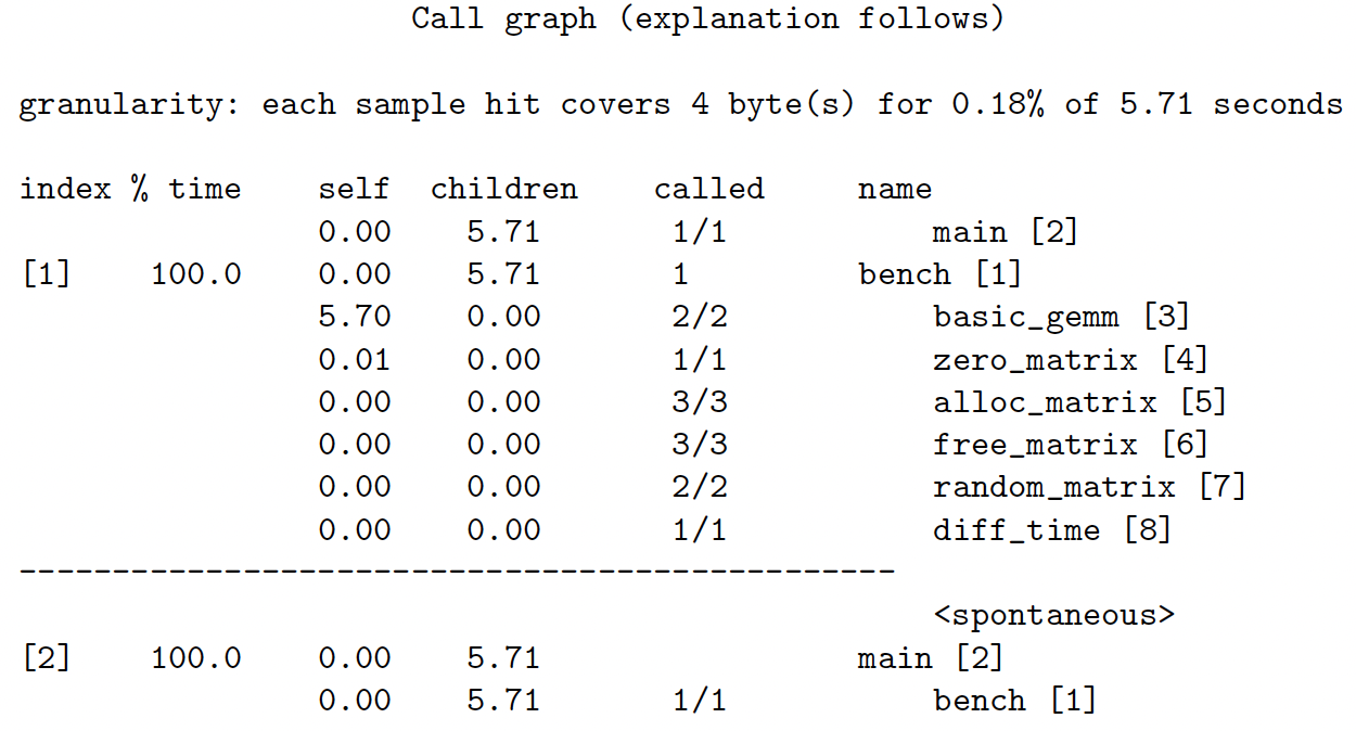
Output: the call graph

Annotated source

static void tiled_packed_gemm(int m, int n, int k,
                               const double * restrict a, int lda,
                               const double * restrict b, int ldb,
                               double * restrict c, int ldc) 
{
    const int ilm = (m / TILESIZE) * TILESIZE;
    const int jlim = (n / TILESIZE) * TILESIZE;
    const int plim = (k / TILESIZE) * TILESIZE;
    ...
}

static void alloc_matrix(int m, int n, double **a) 
{
    ...
}

Optimisation workflow

1. Identify hotspot functions
2. Find relevant bit of code
3. Determine algorithm
4. Add instrumentation markers (see exercise)
5. Profile with more detail/use performance models.

Exercise 6: Finding the hotspot

1. Split into small groups
2. Download the miniMD application
3. Profile with gprof
4. Annotate hotspot with likwid Marker API
5. Measure operational intensity
6. Ask questions!