Robotics 8 Path Planning

Posted Nov 25, 2024 Updated Nov 26, 2024

10 min read

Lecture: Learning Objectives

The aim of this lecture is to design path planning for robot navigation.

Objectives:
1. Obstacle avoidance
2. Search algorithms
- Breadth-first
- Depth-first
- Wavefront
1. Dijkstra’s Algorithm
2. A* Algorithm

Navigation

There are two primary scenarios for robot navigation:

– Known environment

– Unknown environment

For a known environment, a full spatial model (map) exists and the task becomes a search for a path (trajectory) to an end goal.

This can becomes more complicated if the environment is dynamic (obstacles move).

In an unknown environment, no map exists so the challenge is more focused on complete exploration of the area.

Path Planning

Given a complete map of an environment and a target location,

path planning is the process of identifying (searching for) a

geometric path which will get the robot to the goal (kinematics).

Trajectory planning is the process of applying a time constraint to

the path.

Search algorithm performance is measured in a number of

ways:

Completeness
Optimality
Time Complexity
Space Complexity

Obstacle Avoidance

Robot needs to navigate through the environment without running into obstacles.
Robot needs to utilize exteroceptive sensors to identify obstacles.
Example of exteroceptive sensors are: camera, LiDAR, sonar, etc…

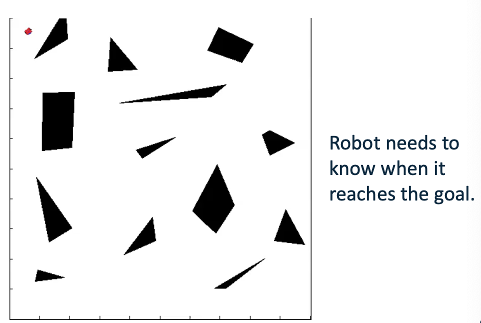
The bug algorithm:

known direction to goal
- robot can measure distance d(x,y) between pts x and y
otherwise local sensing walls/obstacles

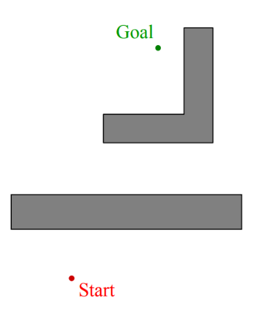
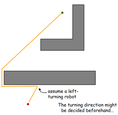
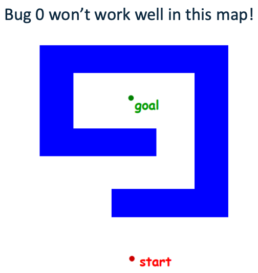
Bug 0 Strategy

head toward goal
follow obstacles until you can head toward the goal again
continue

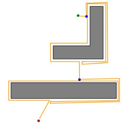
Bug 1 Strategy

Improve algorithm by adding memory!

head toward goal
if an obstacle is encountered, circumnavigate it and remember how close you get to the goal
return to that closest point (by wall-following) and continue

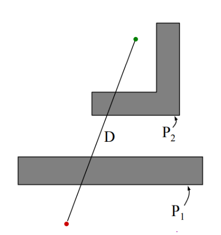
Bug 1 Path Bound

D = straight-line distance from start to goal

Pi = perimeter of the i th obstacle

Lower bound: $D$

What’s the shortest distance it might travel?

Upper bound: $D+1.5\sum_iP_i$

What’s the longest distance it might travel?

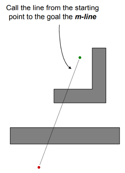
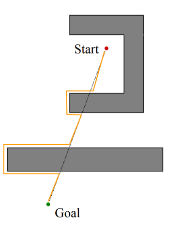
Bug 2 Strategy

head toward goal on the m-line
if an obstacle is in the way, follow it until you encounter the m-line again.(closer to the goal)
Leave the obstacle and continue toward the goal

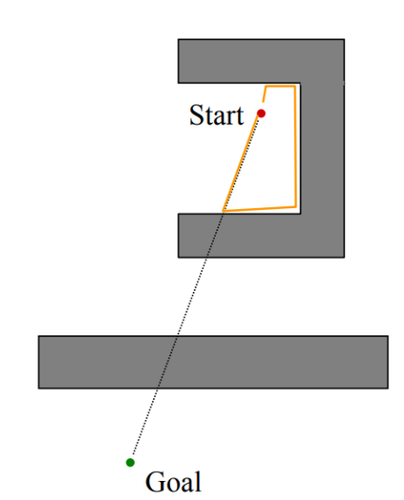
In this case, re-encountering the m-line brings you back to the start
Implicitly assuming a static strategy for encountering the obstacle (“always turn left”)

Bug 2 Path Bound

D = straight-line distance from start to goal

Pi = perimeter of the i th obstacle

Lower bound:$D$

What’s the shortest distance it might travel?

Upper bound:$D+1.5\sum_i\frac{n_i}{2}P_i$

What’s the longest distance it might travel?

𝑛𝑖 = # of m-line intersections of the i th

obstacle

Bug 1 VS Bug 2

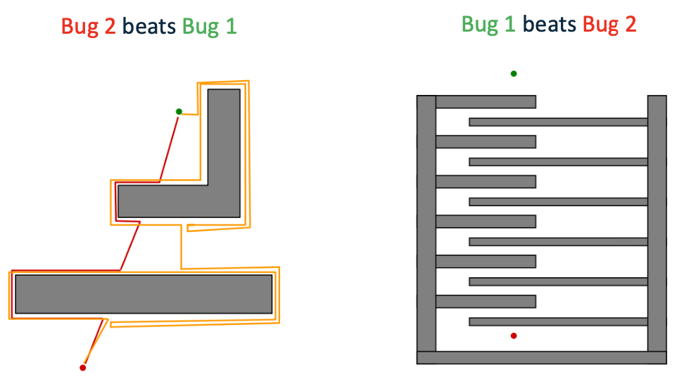
BUG 1 is an exhaustive search algorithm – it looks at all choices before commiting
BUG 2 is a greedy algorithm – it takes the first thing that looks better
In many cases, BUG 2 will outperform BUG 1, but
BUG 1 has a more predictable performance overall

Configuration Space

Mobile robots operate in either a 2D or 3D Cartesian workspace with between 1 and 6 degrees of freedom.

The configuration of a robot completely specifies the robot’s location.

The configuration of a robot, C, with 𝑘 DOF can be described with 𝑘 values: C = {𝑞1, 𝑞2, … , 𝑞𝑘}.

These values can be considered a point, 𝑝 in a k-dimension space (C-space).

C-Space

Wheeled mobile robots can be modelled in such a way that the C-Space maps almost directly to the workspace. $𝐶 = 𝑥, 𝑦, 𝜑$ The assumption is often made that the robot is holonomic, however this is not the case for differential drive robots. If the orientation of the robot is not important, this assumption is valid.

C-Space for Mobile Robots

If we assume a circular, holonomic robot, the C-space of a mobile robot is almost identical to the physical space.

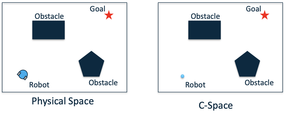
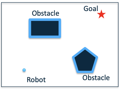
C-Space Modification

The robot in C-space is represented as a point, however the robot in the physical space has a finite size.

To map the obstacles in C-space, they have to be increased in size by the radius of the robot.

Graphs

The standard search methods used for planning a route are based on graphs.

A graph, 𝐺, is an abstract representation which is made up of nodes (Vertices), 𝑉(𝐺), and connections (Edges), 𝐸(𝐺).

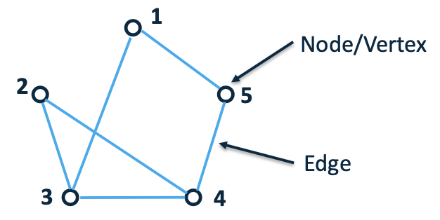
Graph Definitions

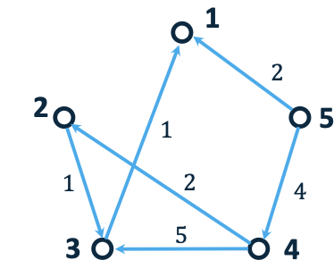
The graph below has a vertex set: $𝑉 (𝐺) = {1,2,3,4,5}$

The degree of a vertex is the number edges with that vertex as an end point (so the degree of node 1 would be 2).

An edge connects two vertices and is defined as (𝑖, 𝑗) i.e. connecting vertex 𝑖 to vertex 𝑗.

The formal definition of the graph is 𝐺 = (𝑉, 𝐸).

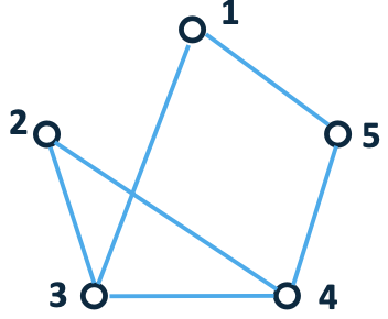
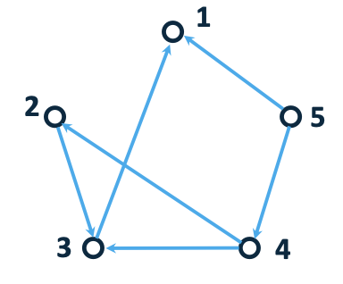
Graph Direction

The previous graph is known as an undirected graph, i.e. you can move from node to node in both directions.

A directed graph means that you can only travel between nodes in a single direction.

Adjacency Matrix

Graphs can be mathematically represented as an adjacency matrix, A, which is a 𝑉 × 𝑉 matrix with entries indicating if an edge exists between them. $a_{ij}=\begin{cases}1&\quad if(i,j)\in E\\0&\quad otherwise\end{cases}$

Example: $\begin{aligned}&a_{12}=a_{21}=\quad0\quad a_{13}=a_{31}=\quad1\quad a_{14}=a_{41}=\quad0\quad a_{15}=a_{51}=\quad1\\&a_{23}=a_{32}=\quad1\quad a_{24}=a_{42}=\quad1\quad a_{25}=a_{52}=\quad1\\&a_{34}=a_{43}=\quad1\quad a_{35}=a_{53}=\quad0\\&a_{45}=a_{54}=\quad1\end{aligned}$

Grid movement

The cell decomposition method approaches the path-planning problem by discretising the environment into cells; each cell can either be an obstacle or free space. Then, a search algorithm is employed to determine the shortest path though these cells to go from the start position to the goal position. This strategy tends to work well in dense environments and some of its algorithms can handle changes in the environment efficiently.

The environment of the robot is a continuous structure that is perceived by the robot sensors. Storing and processing this complex environment in a simple format can be quite challenging. One way to simplify this problem is by discretising the map using a grid. The grid discretises the world of the robot into fixed-cells that are adjacent to each other.

Grid-based discretisation results in an approximate map of the environment. If any part of the obstacle is inside a cell, then that cell is occupied; otherwise, the cell is considered as free space.

Types of Search Algorithms

Search algorithms can be broadly placed into two categories:

Uninformed

– E.g. Breadth-First, Depth-First, Wavefront

Informed

– E.g. Dijkstra, A, D, variants of both

Uninformed searches have no additional information about the environment.

Informed searches have additional information through the use of evaluation functions or heuristics.

Breadth-First Pseudo-Code

A basic search algorithm is called Breadth-First which begins at a start node and searches all adjacent nodes first. It then progresses onto the next ‘level’ node and searches all nodes on that level before it progresses. It terminates when it reaches its goal.

This search method provides an optimal path on the assumption that the cost of traversing each edge is the same.

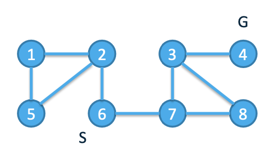
Breadth-First Example

Start Node: 6

End Node: 4

Distance to Node = 3

Path to Node:

6 -> 7 -> 3 -> 4

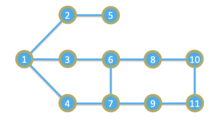
Breadth-First Exercise

\What is the shortest distance to the goal and what is the route?

Start Node: 1

End Node: 11

Depth-First Search

DFS is similar to BSF, however the algorithm expands the nodes to the deepest level first.

There is some redundancy in that the algorithm may have to backtrack to previous nodes.

Depth-First Exercise

What is the shortest distance to the goal and what is the route?

Start Node: 1

End Node: 11

Wavefront Propagation Pseudo Code

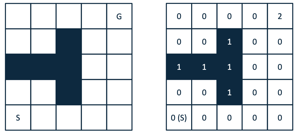
Wavefront Propagation

Start with a binary grid; ‘0’’s represent free space, ‘1’’s represent obstacles
Set the value of the goal cell to ‘2’
Set all ‘0’-valued grid cells adjacent to the ‘2’ cell with ‘3’
Set all ‘0’-valued grid cells adjacent to the ‘3’ cell with ‘4’
Continue until the wave front reaches the start cell (or has populated the whole grid)

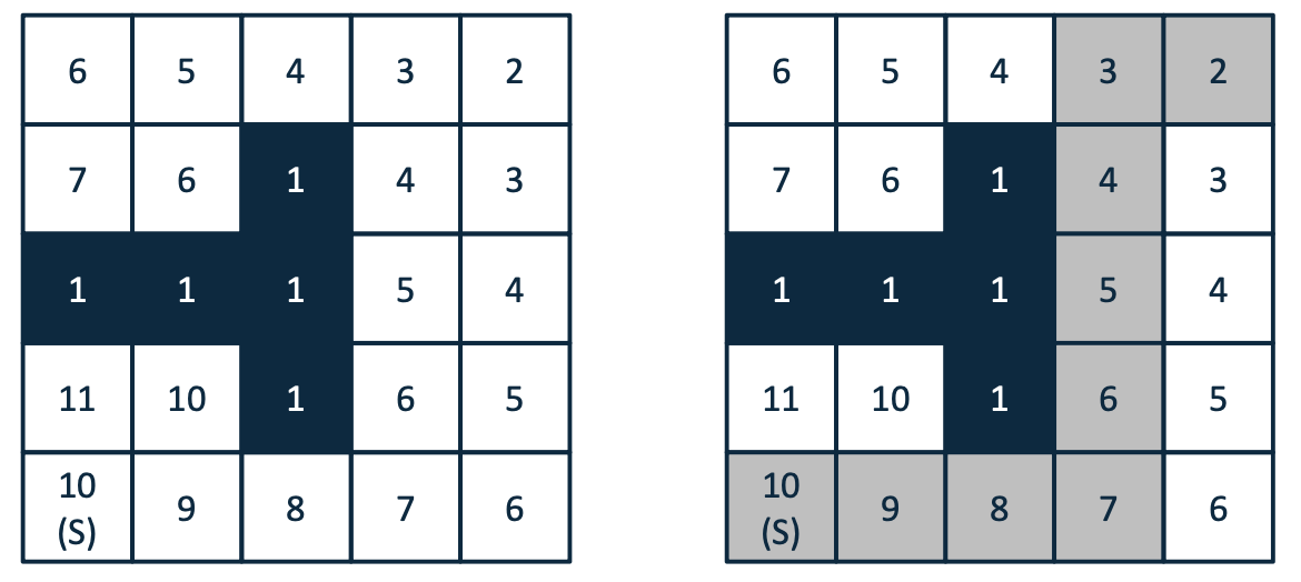
Extract the path using gradient descent

Given the start cell with a value of ‘x’, find the neighbouring grid cell with a value ‘x-1’. Add this cell as a waypoint.
From this waypoint, find the neighbouring grid cell with a value ‘x-2’. Mark this cell as a waypoint.
Continue until you reach the cell with a value of ‘2’

Wavefront Example

Dijkstra’s Algorithm

Up till now, the edges of the graphs we have considered have all had the same weight. As observed in the previous example, this doesn’t necessarily provide the optimal route.

Dijkstra’s algorithm is similar to the BFS, however edges can take any positive cost.

This algorithm finds the costs to all vertices in the graph rather than just the goal.

This is an informed search where the node with the lowest $𝑓(𝑛)$ is explored first. 𝑔(𝑛) is the distance from the start. $𝑓(𝑛) = 𝑔(𝑛)$

Dijkstra Pseudo Code

Initialise vectors

a. Distance to all other nodes, 𝑓[𝑛] = Inf

b. Predecessor vector (pred) = Nil (0)

c. Priority vector, Q

For all nodes in the graph
1. Find the one with the minimum distance
2. For each of the neighbour nodes
  i. If the distance to the node from the start is shorter, update the path distance (if 𝑓[𝑢] + 𝑤(𝑢, 𝑛) < 𝑓[𝑛])
Find the path to the goal based on the shortest distances

Dijkstra Example

Node	1	2	3	4
1	0	0	0	0
2	0	0	1	0
3	1	0	0	0
4	0	2	5	0
5	2	0	0	4

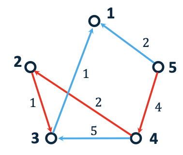
Start: 5, Goal: 3

Shortest Path = 7

Path = 5 -> 4 ->2 -> 3

**A* Search Algorithm** (考试会考)

One of the most popular search algorithms is called A* (A-star) A* uses heuristics, additional information about the graph, to help find the best route. $𝑓 (𝑛) = 𝑔 (𝑛) + ℎ (𝑛)$ 𝑛 is the node

𝑔(𝑛) is the distance from the start node to 𝑛

ℎ(𝑛) is the estimated distance to the goal from 𝑛

Nodes with the lowest cost are explored first.

Heuristics

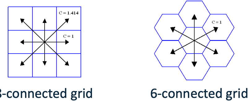
For grid maps, the heuristic function can be calculation a number of ways depending on the type of movement allowed.

von Neumann – Manhattan Distance
Moore – Octile or Euclidean Distance

The heuristic function should be ‘admissible’, i.e. always underestimate the distance to the goal: $ℎ (𝑛) ≤ ℎ^∗ (𝑛)$

**A* Pseudo Code**

Initialise vectors
a. Distance to all other nodes, 𝑓[𝑛] = Inf
b. Predecessor vector (pred) = Nil (0)
c. Priority vector, Q
From the starting node to the end node
a. Find the node with the minimum 𝑓(𝑛). If there is more than one with the same value, select the node with the smallest ℎ(𝑛)
b. For each of the neighbour nodes
i. If 𝑓(𝑛) is smaller, update the path distance $𝑔[𝑢] + 𝑤(𝑛, 𝑢) + ℎ(𝑛) < 𝑓[𝑛]$
Find the path to the goal based on the shortest distances

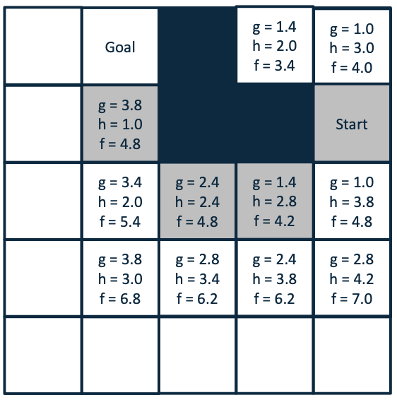
**A* Example**

Using Octile Distances and Moore Movement.

Advanced Planning Algorithms

There are more advanced planning algorithms which increase

performance and can operate in dynamic conditions:

Anytime Replanning A*
D*
Anytime D*
Potential Fields

Study, Master

DU Robotics

This post is licensed under CC BY 4.0 by the author.