Robotics 6 Localisation
RP6 Localisation
Objectives:
- Differential drive robots
- Localisation
- Motion control
book: Introduction to Mobile Robot Control, Spyros G. Tzafestas, 2014
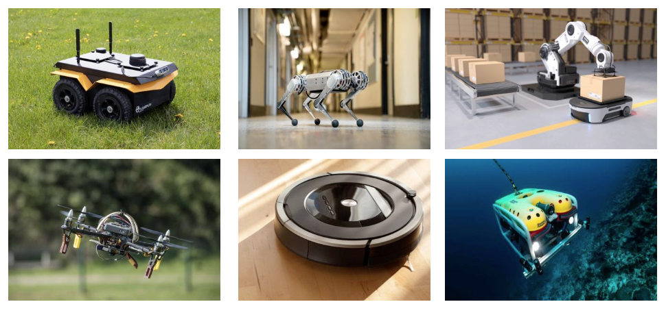
Mobile robots
- A robot is an artificial physical agent that perceives its environment through sensors and acts upon that environment through actuators
Driving robot around?
- What does it take to drive a robot from point A to B?
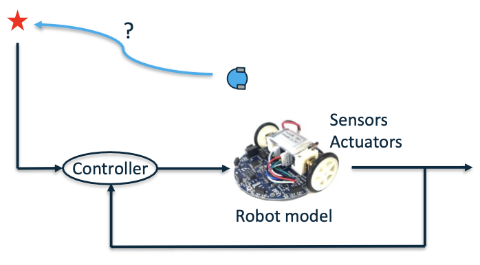
– self control self decision
Divide and Conquer 分而治之
The world is dynamic and fundamentally unknown
The controller must be able to respond to environmental conditions
Instead of building one complicated controller – divide and conquer: Behaviors
➢ Go-to-goal
➢ Avoid-obstacles
➢ Follow-path
➢ Track-target
➢ …
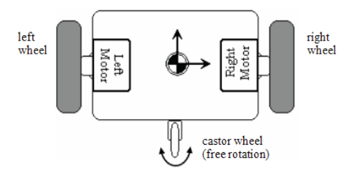
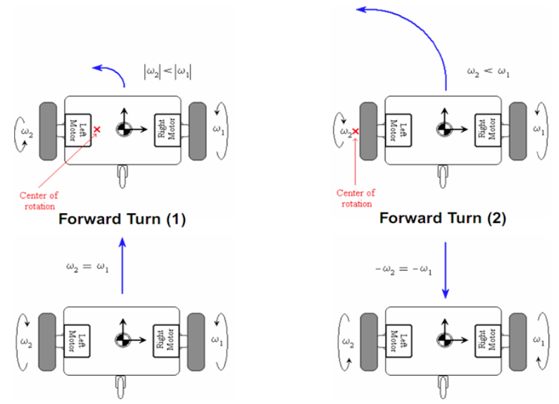
Differential drive robots
- Also known as differential wheeled robots(差速轮式机器人), these are mobile robots whose movement is based on two separately driven wheels placed on either side of the robot body. It can thus change its direction by varying the relative rate of rotation of its wheels, thereby requiring no additional steering motion.
**Differential drive **kinematics(运动学)
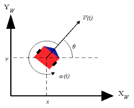
Kinematics of a unicycle
Ignoring balancing concerns, there are two action variables, i.e., direct inputs to the system in the 𝑋𝑌 plane.
• The first one is the forward/linear velocity: $𝑣=𝜔_𝑢𝑟$, where $𝜔_𝑢$ is the wheel angular velocity, 𝑟 is wheel radius
• The second one is the steering velocity denoted by 𝜔.
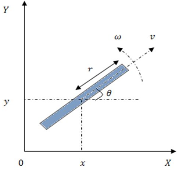
Dynamics: \(\begin{aligned}&\dot{x}=v\cdot\mathrm{cos}\theta\\&\dot{y}=v\cdot\mathrm{sin}\theta\\&\dot{\theta}=\omega\end{aligned}\) The nonholonomic constraint: \(\dot{x}\mathrm{sin}\theta-\dot{y}\mathrm{cos}\theta=0\) 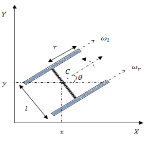
- The resultant forward velocity through 𝐶 (the centre of mass) is $v=r(\frac{\omega_r+{\omega_l}}2)$.
The steering velocity is $\omega=r(\frac{\omega_r-{\omega}_l}l)$.
- Thus, just like the unicycle, the configuration transition equations may be given as
- Comparing the equations for unicycle and for differential drive yields the transformation $v,\omega$ 矩阵化表达 \(\begin{bmatrix}v\\\omega\end{bmatrix}=\begin{bmatrix}r/_2&r/_2\\r/_l&-^r/_l\end{bmatrix}\begin{bmatrix}\omega_r\\\omega_l\end{bmatrix}\)
Localisation
- The robot needs to know its location in the environment in order to make proper decisions.
- Localisation can be achieved using:
- Proprioceptive sensors (encoders, IMU). This type of localisation is named dead reckoning localisation.
- Exteroceptive sensors (sonar, LiDAR, camera). This type of localisation is named map-based localisation.
- External sensors (GPS). Not suitable for indoor applications.
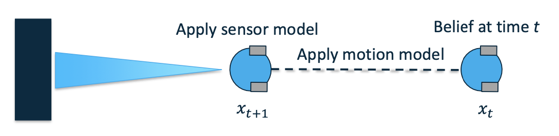
Probabilistic Localisation
- In robotics, we deal with localization probabilistically
- Three key components:
- A robot’s belief of where it is (its state)
- A robot’s motion model
- A robot’s sensor model
Motion-based Localisation(Dead Reckoning)
This technique uses the internal kinematics of the robot to localise it in the environment.
This method is simple to implement, and does not require sophisticated sensors.
However, such technique suffers from the unbounded growth of uncertainty about the robot pose over time due to the numerical integration and accumulation of error.
@Vergil
- The robot needs to know its location in the environment in order to make proper decisions
- Localisation can be achieved using
- Proprioceptive sensors(encoders, IMU). This types of localisation is named dead reckoning localisation.
- Exteroceptive sensors(sonar, LiDAR, camera). This type of localisation is named map-based localisation
- External sensors(GPS). Not suitable for indoor applications
Probabilistic Localisation
- In robotics, we deal with localisation probabilistically
- Three key components:
- A robot’s belif of where it is (its state)
- A robot’s motion model
- A robot’s sensor model
Motion-based Localisation(Dead Reckoning)
This technique uses the internal kinematics of the robot to localise it in the environment.
This method is simple to implement, and does not require sophisticated sensors.
However, such technique sufers from the unbounded growth of the uncertainty about the robot pose over time due to the numerical integration and accumulation of Error
Kinematic model for a differential robot model \(\frac{d}{dt} \begin{bmatrix} s_x \\ s_y \\ s_\theta \end{bmatrix} = \begin{bmatrix} \cos(s_\theta) & 0 \\ \sin(s_\theta) & 0 \\ 0 & 1 \end{bmatrix} \begin{bmatrix} v \\ \omega \end{bmatrix}\)
The robot pose \(\mathbf{s}_k=\begin{bmatrix}s_x&s_y&s_\theta\end{bmatrix}^T\)
The robot inputs \(\mathbf{u}_k=\begin{bmatrix}v&\omega\end{bmatrix}^T\)
If $\Delta t$ is the sampling time , then it is possible to compute the incremential linear and angular Displacement, $\Delta d$ and $\Delta \theta$, as follows: \(\begin{aligned}&\Delta d=v\cdot\Delta t\quad\Delta\theta=\omega\cdot\Delta t\\&\begin{bmatrix}\Delta d\\\Delta\theta\end{bmatrix}=\begin{bmatrix}1/2&1/2\\1/l&-1/l\end{bmatrix}\begin{bmatrix}\Delta d_r\\\Delta d_l\end{bmatrix}\end{aligned}\)
To compute the pose of the robot at any given time step, the kinematic model must be numerically integrated.
This approximation follows the Markov assumption where the current robot pose depends only on the previous pose and the input velocities \(\begin{bmatrix}S_{x,k}\\S_{y,k}\\S_{\theta,k}\end{bmatrix}=\begin{bmatrix}S_{x,k-1}\\S_{y,k-1}\\S_{\theta,k-1}\end{bmatrix}+\begin{bmatrix}\Delta d\cos\bigl(s_{\theta,k-1}\bigr)\\\Delta d\sin\bigl(s_{\theta,k-1}\bigr)\\\Delta\theta\end{bmatrix}=\begin{bmatrix}S_{x,k-1}\\S_{y,k-1}\\S_{\theta,k-1}\end{bmatrix}+\begin{bmatrix}v\Delta t\cos\bigl(s_{\theta,k-1}\bigr)\\v\Delta t\sin\bigl(s_{\theta,k-1}\bigr)\\ \omega \Delta t\end{bmatrix}\)
The pose estimation of a mobile robot is always associated with some uncertainty with respect to its state parameters.
From a geometric point of view, the error in differential-drive robots is classified into three groups:
- Range error: it is associated with the computation of $\Delta d$ over time
- Turn error: it is associated with the computation of $\Delta \theta$ over time
- Drift error: it is associated with the difference between the angular speed of the wheels and it affects the error in the angular rotation of the robot.
Due to such uncertainty, it is possible to represent the belief of the robot pose by a Gaussian distribution, where
- the mean vector $\mu_k$ is the best estimate of the pose, and
- the covariance matrix $\sum_k$ is the uncertainty of the pose that encapsulates the erros presented in the previous slide
The Guassian distribution (or normal distribution) is denoted by \(\mathbf{s}_k{\sim}\mathcal{N}(\mathbf{\mu}_k,\mathbf{\Sigma}_k).\)
Gaussian Distributions
A random varibale $X$ is noramlly distributed, or Gaussian, if its probability density function is defined as: \(p_X(x)=\frac{1}{\sqrt{2\pi\sigma^2}}exp\left(-\frac{(x-\mu_X)^2}{2\sigma^2}\right)\) where, $\mu_X, \sigma^2$ are the mean and variance, respectively; they are the distribution parameters. The notation $X \sim \mathcal{N} (\boldsymbol{\mu}_X,\boldsymbol{\Sigma}_X)$ means that the random variable $X$ is Gaussian.
Affine Transformation
Consider $X \sim \mathcal{N} (\boldsymbol{\mu}_X,\boldsymbol{\Sigma}_X)$ in $\R^n$, and let $Y = \mathbf{A}X + \boldsymbol{b}$ be the affine transformation, where $\mathbf{A} \in \R^{m \times n}$ and $\mathbf{b} \in \R^m$. Then, the random vector $Y \sim \mathcal{N} (\boldsymbol{\mu}_X,\boldsymbol{\Sigma}_Y)$ such that: \(\begin{aligned}\boldsymbol{\mu}_Y&= \mathbf{A}\boldsymbol{\mu}_X + \mathbf{b}\\\\\boldsymbol{\Sigma}_Y&=\mathbf{A}\boldsymbol{\Sigma}_X\mathbf{A}^T\end{aligned}\)
In the context of probability, the robot pose at time step $k$, denoted by $s_k$, can be described with Markov assumption as function of previous robot pose $s_{k-1}$ and the current control input $\mathbf{u}{k}=[v{k}\quad\omega_{k}]^{T}$. This process is called the robot motion model. \(\mathbf{s}_k=\mathbf{h}(\mathbf{s}_{k-1},\mathbf{u}_k)+\mathbf{q}_k\) where $q_k$ is an additive Gaussian noise such that $\mathbf{q}_k{\sim}\mathcal{N}(\mathbf{0},\mathbf{Q}_k)$, and $Q_k$ is a positive semidefinite covariance matrix.
The function $\mathbf{h}(\mathbf{s}_{k-1},\mathbf{u}_k)$ is generally nonlinear, and in the case of a differential-drive robot, this fucntion is defined as: \(\mathbf{h}(\mathbf{s}_{k-1},\mathbf{u}_{k})=\begin{bmatrix}s_{x,k-1}+\Delta t\cdot v_k.\cos\bigl(s_{\theta,k-1}\bigr)\\s_{y,k-1}+\Delta t\cdot v_k.\sin\bigl(s_{\theta,k-1}\bigr)\\s_{\theta,k-1}+\Delta t\cdot\omega_k\end{bmatrix}\)
Assume that the robot pose at time step $k - 1$ is given by a Gaussian distribution such that $\mathbf{s}{k-1}{\sim}\mathcal{N}(\boldsymbol{\mu}{k-1},\boldsymbol{\Sigma}_{k-1})$
Then, the above setup can be used to estimate the robot pose at time step k by linearising the robot motion model using first-order Taylor expansion around $\mu_k$ as follows \(\mu_k=\mathbf{h}(\mu_{k-1},\mathbf{u}_k)\)
The following equation represents the Jacobian matrix of $\mathbf{h}(\mu_{k-1},\mathbf{u}k)$ with respect to each variable in $s{k-1}$, evaluated at $s_{k-1} = \mu_{k-1}$ \(\mathbf{H}_{k}=\nabla_{\mathbf{s}_{k}}\mathbf{h}(\mathbf{s}_{k-1},\mathbf{u}_{k})\Big|_{\mathbf{s}_{k-1}=\mu_{k-1}}\) and the pose $s_k$ is computed using the linearised system: \(\mathbf{s}_k\approx\mathbf{\mu}_k+\mathbf{H}_k(\mathbf{s}_{k-1}-\mathbf{\mu}_{k-1})\)
In the case of a differential-drive robot, the Jacobian $H_k$ is computed as follows: \(\mathbf{h}(\mathbf{s}_{k-1},\mathbf{u}_k)=\begin{bmatrix}s_{x,k-1}+\Delta t\cdot v_k.\cos(s_{\theta,k-1})\\s_{y,k-1}+\Delta t\cdot v_k.\sin(s_{\theta,k-1})\\s_{\theta,k-1}+\Delta t\cdot\omega_k\end{bmatrix}\)
\[\begin{gathered}\mathbf{H}_{k}=\begin{bmatrix}\frac{\partial h_1}{\partial s_{x,k}}&\frac{\partial h_1}{\partial s_{y,k}}&\frac{\partial h_1}{\partial s_{\theta,k}}\\\frac{\partial h_2}{\partial s_{x,k}}&\frac{\partial h_2}{\partial s_{y,k}}&\frac{\partial h_2}{\partial s_{\theta,k}}\\\frac{\partial h_3}{\partial s_{x,k}}&\frac{\partial h_3}{\partial s_{y,k}}&\frac{\partial h_3}{\partial s_{\theta,k}}\end{bmatrix}\\=\begin{bmatrix}1&0&-\Delta t\cdot v_k\cdot\sin(\mu_{\theta,k-1})\\0&1&\Delta t\cdot v_k\cdot\cos(\mu_{\theta,k-1})\\0&0&1\end{bmatrix}\end{gathered}\]Since the robot motion model is linearised and all uncertainties are Gaussians, it is possible to compute the covariance $\Sigma_k$ associated with the robot pose at time step $k$ using the properties of Gaussians: \(\Sigma_k = H_k \Sigma_{k-1} H_k^T + Q_k\)
Thus, the estimated pose at time step $k$ is Gaussian such that $s_k \sim \mathcal{N}(\mu_k, \Sigma_k)$, and it is computed recursively using the pose at time step $k - 1$ and the input vector $\mathbf{u_k}$. The initial robot pose is assumed known such that $\mu_0 = 0$, and $\Sigma_0 = 0$.
The pose uncertainty will always increase every time the robot moves due to the addition of the nondeterministic error represented by $Q_k$, which is positive semi-definite.
The joint uncertainty of $s_x$ and $s_y$ is represented by an ellipsoid around the robot. This ellipsoid is named Ellipsoid of Confidence. As the robot moves along the $x$-axis, its uncertainty along the $y$-axis increases faster than the $x$-axis due to the drift error.
The uncertainty ellipsoid is no longer perpendicular to the motion direction as soon as the robot starts to turn.
Pose covariance matrix
Consider the following motion model for a differential drive robot: \(\boldsymbol{h}\big(\boldsymbol{s}_{k},\omega_{r,k},\omega_{l,k}\big)=\begin{bmatrix}s_{x,k-1}+r\Delta t \frac{\omega_{r,k}+\omega_{l,k}}{2}\cos( s_{\theta,k-1}\big)\\s_{y,k-1}+r\Delta t \frac{\omega_{r,k}+\omega_{l,k}}{2}\sin( s_{\theta,k-1}\big)\\s_{\theta,k-1}+r\Delta t \frac{\omega_{r,k}-\omega_{l,k}}{l}\end{bmatrix}\) where $\omega_{r,k}$ and $\omega_{l,k}$ are the right and left wheel angular velocity at time step keep
Now assume the noise in both right and left wheel angular velocities to be zero-mean Gaussian distribution such that: \(\begin{bmatrix} \omega_{r,k} \\ \omega_{l,k} \end{bmatrix} \sim \mathcal{N}(0, \Sigma_{\Delta,k})\)
\[\Sigma_{\Delta,k} = \begin{bmatrix} k_r |\omega_{r,k}| & 0 \\ 0 & k_l |\omega_{l,k}| \end{bmatrix}\]where $k_r$ and $k_l$ are constants representing the error associated with computing the angular velocity by each wheel.
These constants are related to the traction between the wheels and the floor surface or the encoder noise used to compute the wheel displacements.
Larger angular speed of the right motor $ \omega_{r,k} $ will lead to a larger variance of that motor $k_r \omega_{r,k} $. - It is possible to propagate this noise $\Sigma_{\Delta, k}$ to be seen from the robot state prospective using Taylor series expansion as follows:
Motion Control
The motion control for a mobile robot deals with the task of finding the control inputs that need to be applied to the robot such that a predefined goal can be reached in a finite amount of time.
Control of differential drive robots has been studied from several points of view, but essentially falls into one of the following three categories: point- to-point navigation (or point stabilisation), trajectory tracking, and path following.
The objective here is to drive the robot to a desired fixed state, say a fixed position and orientation. Point stabilisation presents a true challenge to control system when the vehicle has nonholonomic constraints, since that goal cannot be achieved with smooth time-invariant state-feedback control laws. This control technique will be used in this course.
The objective is driving the robot into following a time-parameterised state trajectory. In fact, the trajectory tracking problem for fully actuated systems is well understood and satisfactory solutions can be found in advanced nonlinear control textbooks. However, in case of underactuated systems, the problem is still a very active area of research.
In this case the vehicle is required to converge to and follow a path, without any temporal specifications. The underlying assumption in path following control is that the vehicle’s forward speed tracks a desired speed profile, while the controller acts on the vehicle orientation to drive it to the path. Typically, smoother convergence to a path is achieved and the control signals are less likely pushed to saturation.
Point Stabilisation
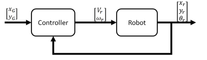
The goal can be defined in the simplest way as a set of coordinates in a multidimensional space. For instance, if the robot is moving in a two dimensional space the goal is:
$X_g=\begin{pmatrix}x_g\y_g\end{pmatrix}$ if the position of the robot needs to be controlled, or
$X_g=\begin{pmatrix}x_g\y_g\\theta_g\end{pmatrix}$ if both position and heading need to be controlled
In order to design the controller we first need to define the robot inputs, robot pose and the goal. For a non-holonomic robot moving in a 2D environment the robot pose can be represented by the vector \(\boldsymbol{\rho}_r=\begin{pmatrix}x_r\\y_r\\\theta_r\end{pmatrix}\) The inputs are the linear and angular velocity of the robot \(v_r=\binom{v_r}{\omega_r}\)
For the sake of simplicity, in this course, the goal is defined only by a 2D set of coordinates $X_g=\begin{pmatrix}x_g\y_g\end{pmatrix}$
Then compute the errors by using the goal coordinates and robot position as in the following: \(e_{x}= x_{g}-x_{r}\\e_{y}= y_{g}-y_{r}\\e_{\theta}= atan2(e_{y},e_{x})-\theta_{r}\)
The robot position is assumed to be known and can be computed using various localisation techniques as Dead Reckoning. The equations for the error can be represented in vector format as follows: \(\boldsymbol{e}=\begin{pmatrix}e_x\\e_y\\e_\theta\end{pmatrix}\) The general form of the control law can be written as: \(\begin{pmatrix} v_r \\ \omega_r \end{pmatrix} = K \begin{pmatrix} e_x \\ e_y \\ e_\theta \end{pmatrix}\) where $K = \begin{pmatrix} k_{11} & k_{12} & k_{13}
k_{21} & k_{22} & k_{23} \end{pmatrix}$, is the control matrix
For simplicity the six controller gain parameters can be reduced to only two by defining the distance error: \(e_d = \sqrt{e_x^2 + e_y^2}\) The control law can now be written as: \(v_r = K_de_d\\ \omega_r = K_\theta e_\theta\)
Closed-loop control block diagram: