Robotics 7 Control

Control

Learning Objectives

The aim of this lecture is to design a control system for dynamical systems.

• Objectives:

1. Feedback Systems
2. Bang-Bang Control
3. PID Control
4. State-Space Representation
5. Stability of the System

Robot Control

• Robot control with (almost) no theory
  • PID Controller
  • Differential drive robots
• Control theory (State-space)
  • Multiple inputs / Multiple outputs
  • Dynamics of internal states

Open-Loop Systems

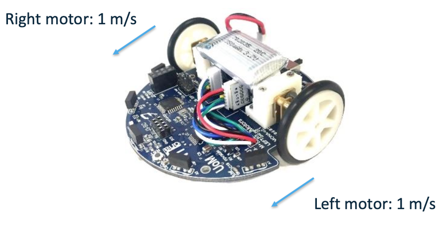
In reality, will the robot move in a straight line at 1 m/s?

Probably NO!

Open-Loop VS Closed-Loop

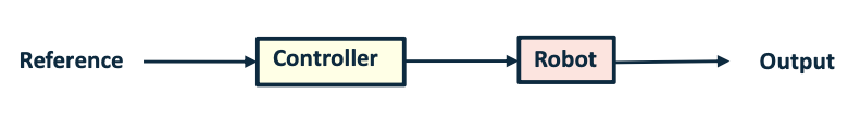
Not using any output ➡ not correct itself

• Easy to implement
• Large tracking error
• Difficult to coordinate

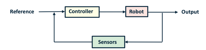
• Accurate motion
• Possible to apply coordination algorithms
• Robust to disturbance
• More efforts in controller design and hardware implementation

Example

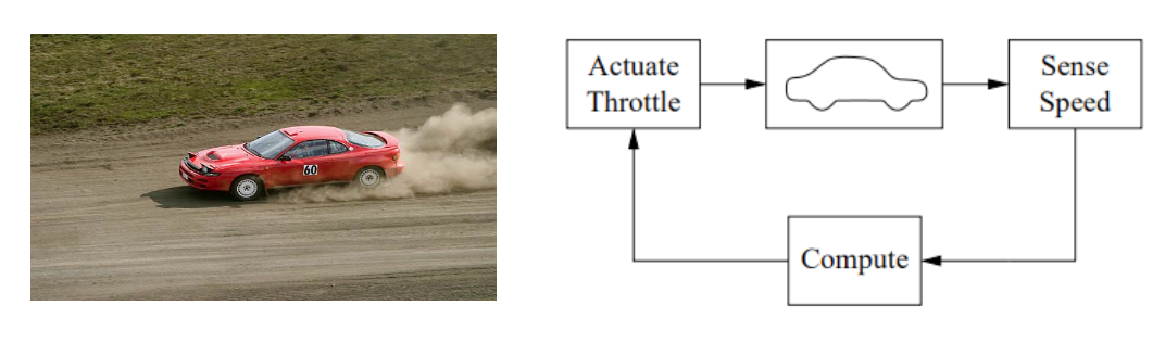
A feedback system for controlling the speed of a vehicle. In the block diagram, the speed of the vehicle is measured and compared to the desired speed within the “Compute” block. Based on the difference in the actual and desired speeds, the throttle (or brake) is used to modify

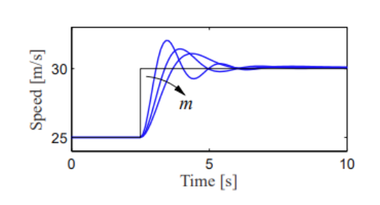
The figure shows the response of the control system to a commanded change in speed from 25 m/s to 30 m/s. The three different curves correspond to differing masses of the vehicle, between 1000 and 3000 kg

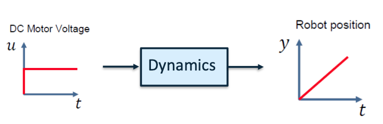
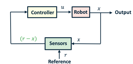
Simple control system

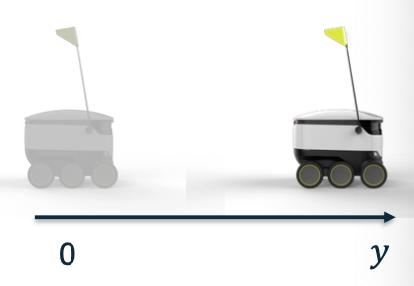
Mobile robot with 1-dimensional motion

• Single Input Single Output (SISO) system
• Input [𝑢]: DC Motor voltage
• Output [𝑦]: robot position

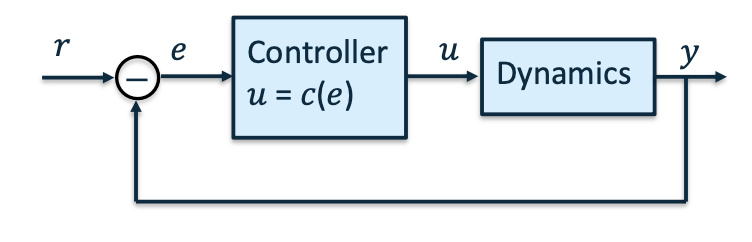
Move robot to position 𝑟

• Reference [𝑟]: The desired value for the output
• Error [𝑒 = 𝑟 − 𝑦]: Difference between desired and actual output.
• Input [𝑢 = 𝑐(𝑒)]: Reacts to the error.

Bang-Bang Control

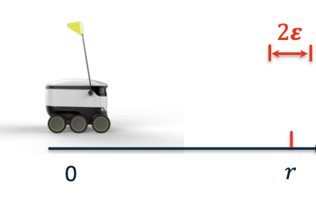$c(e)=\{\begin{array}{ll}u=u_{max},& e>\epsilon \\ u=-u_{max},& e<-\epsilon \\ u=0,& |e|\le \epsilon & \end{array}$

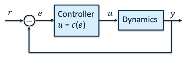
Simulation

$$u_{max}=5\mathrm{V}r=0.5\mathrm{m}\epsilon =1\mathrm{mm}$$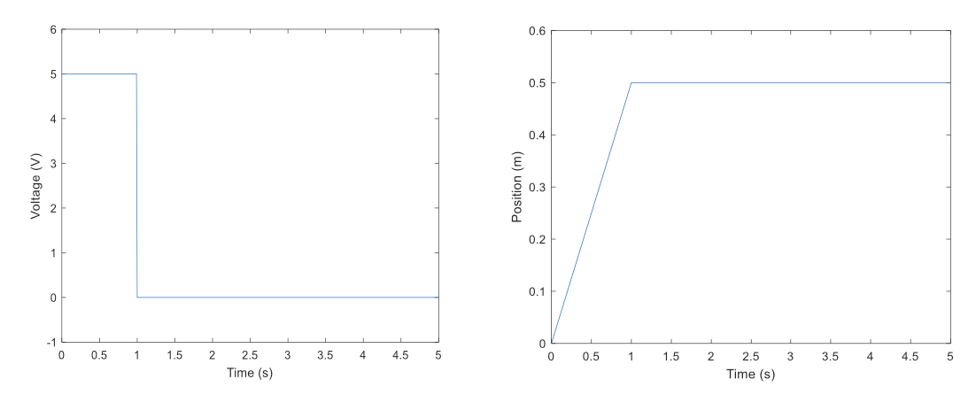

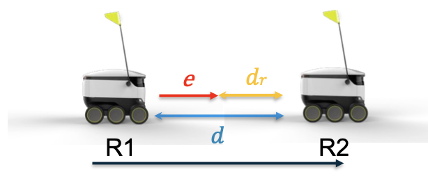
Following Another Robot

Control R1 to keep a constant distance 𝑑𝑟 from R2.

R2 moves at a constant speed 𝑠

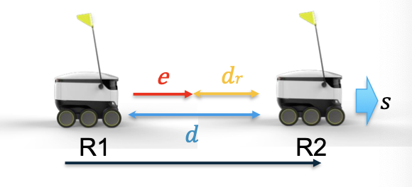
• Input [𝑢]: DC Motor Voltage of R1
• Output [𝑦]: position of R1
• Error [𝑒 = 𝑑−𝑑𝑟]: distance to the desired position

Bang-Bang Control

$c(e)=\{\begin{array}{ll}u=u_{max},& e>\epsilon \\ u=-u_{max},& e<-\epsilon \\ u=0,& |e|\le \epsilon & \end{array}$

Simulation

$$u_{max}=5\mathrm{V}{d}_r=0.5\mathrm{m}\epsilon =1\mathrm{mm}s=0.3\mathrm{m}/\m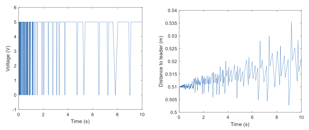athrm{s}$$

Can we make it smoother?

Proportional Control(P in PID)

$c(e)=K_{p}e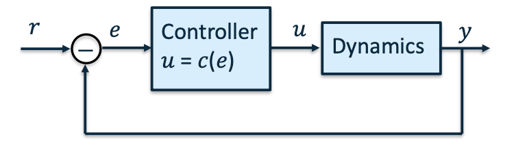$ $K_p=5$

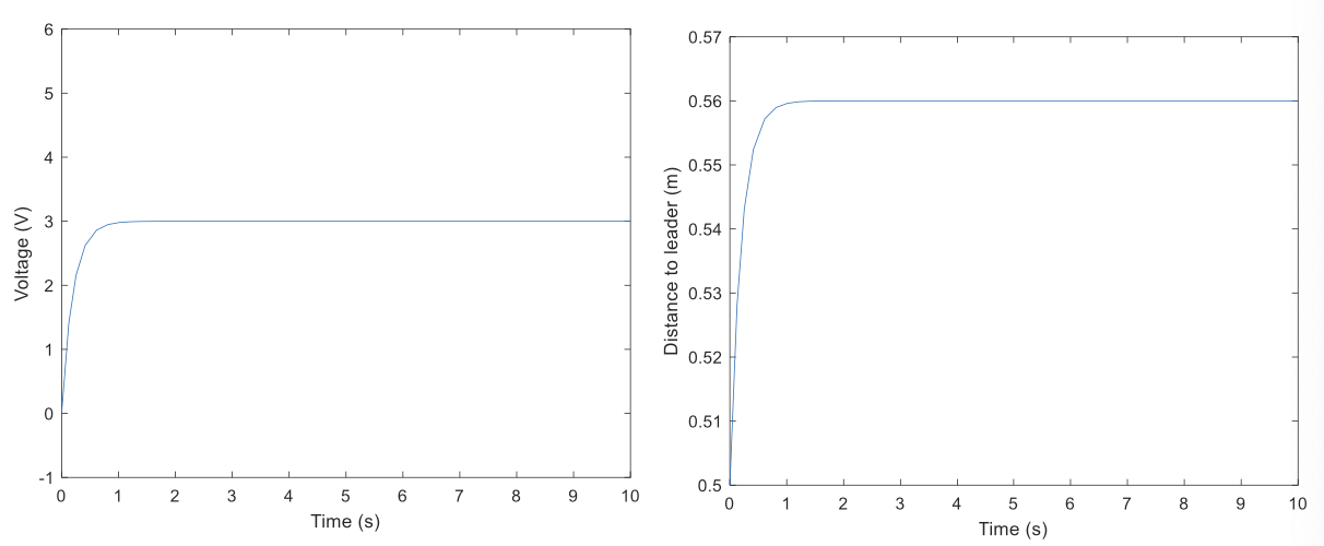
The control is smoother now, but it does not converge to 0.5 !

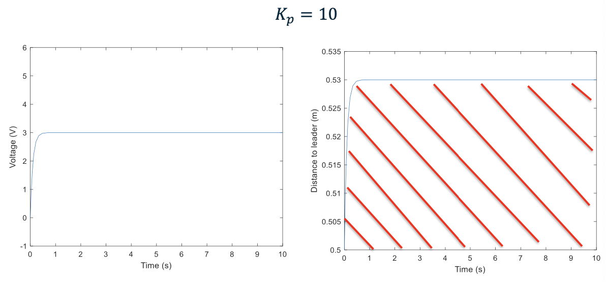
Increase $K_p$

$$K_p=10$$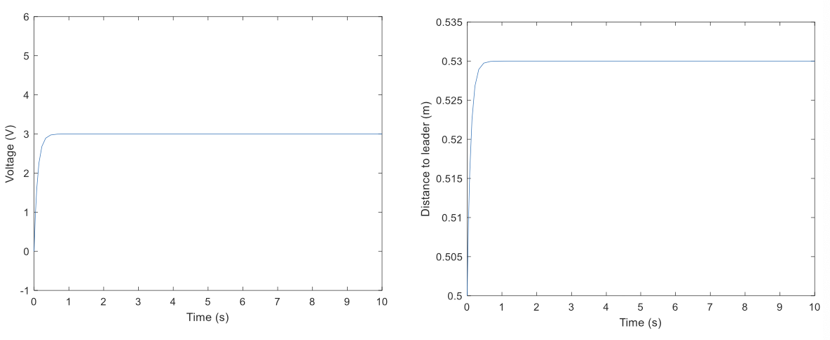

The output is now a little bit closer to 0.5 !

Keep Increase

$K_p=15$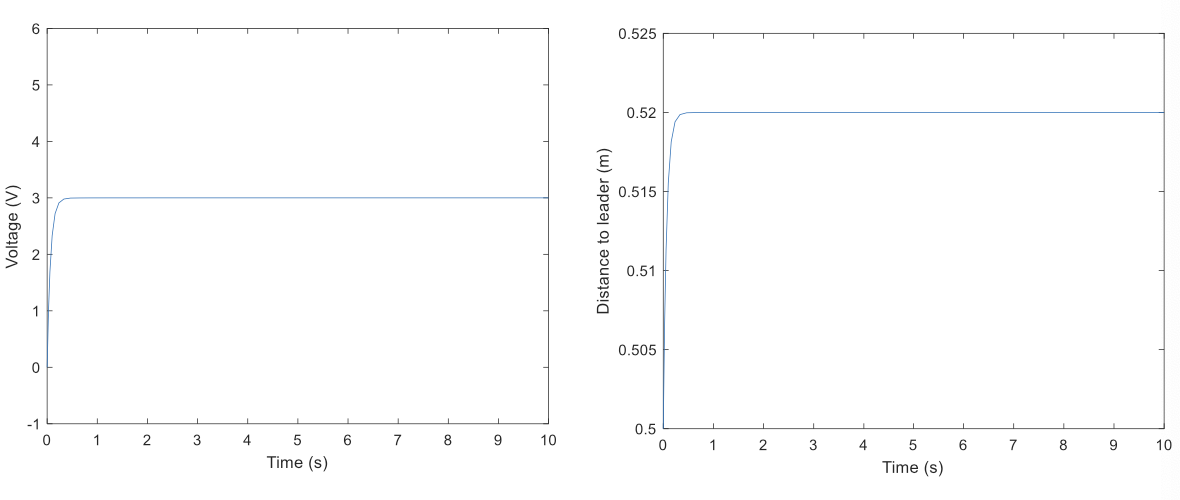

The distance is now further closer to 0.5 !

Keep Increase

$$K_p=100$$

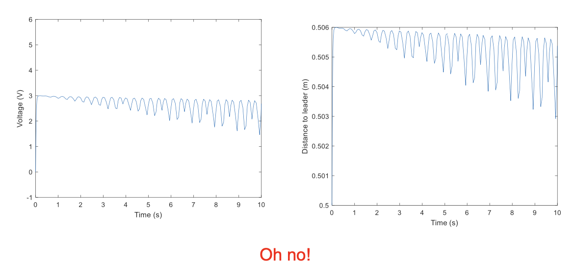
We need to do something different

Proportional–Integral (PI) Control

$c(e)=K_{p}e(t)+K_i{\int }_0^{t}e(t)dt$

PI Control

$$K_p=10K_i=10$$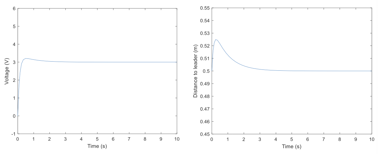

The output converges to 0.5, but it takes longer time

$K_p=10K_i=50$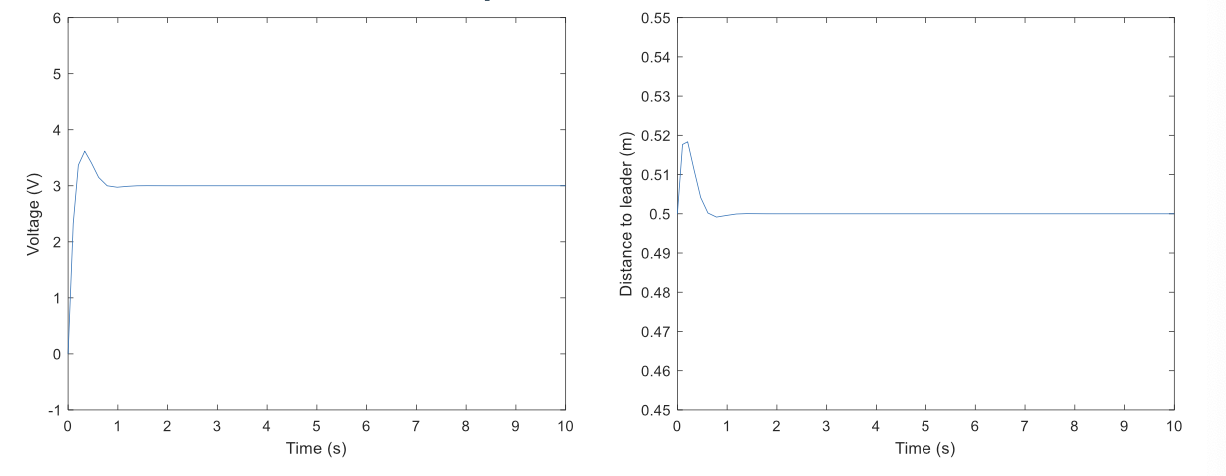

The settling time is shorter

$K_p=10K_i=500$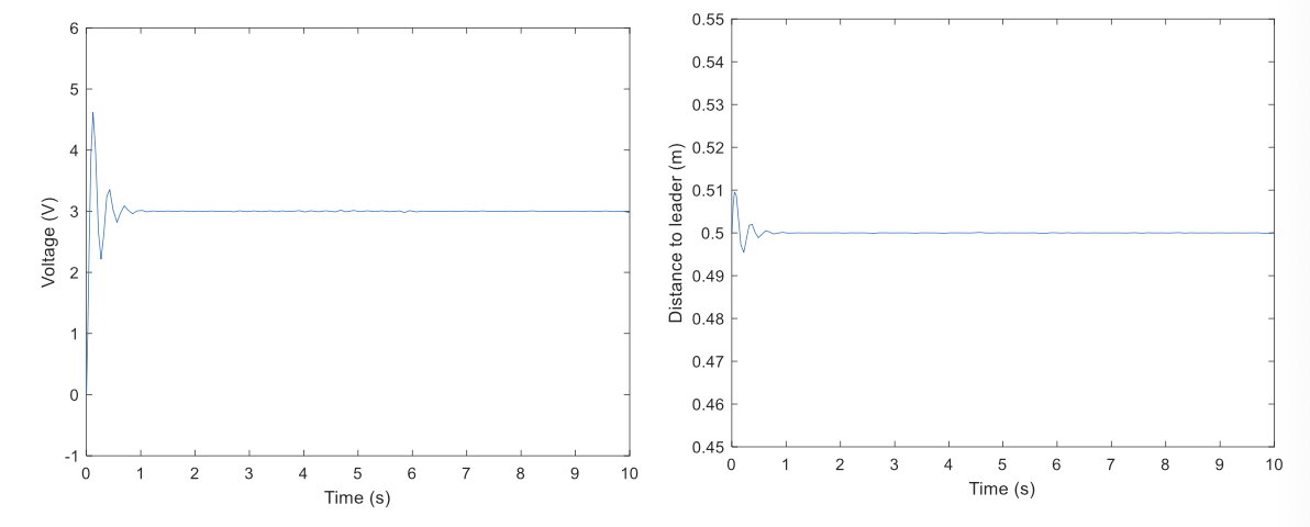

Oh no! It is oscillating again!

Proportional-Integral-Derivative (PID) Control

$c(e)=K_{p}e(t)+K_i{\int }_0^{t}e(t)dt+K_d\frac{d}{dt}e(t)$

P current

I past

D predict future

???

PID Control

$$K_p=10K_i=50K_d=10$$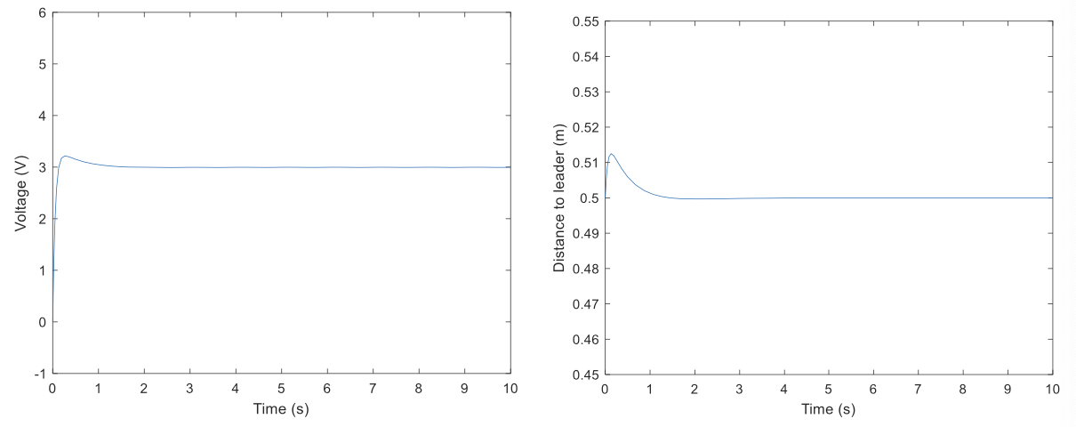

The performance looks good in simulation, but would this work well in a real system?

Summary of Tuning Tendencies

Response	Rise Time	Overshoot	Settling Time	Steady-State Error
$K_p$	Decrease	Increase	Small change	Decrease
$K_i$	Decrease	Increase	Increase	Eliminate
$K_D$	Small change	Decrease	Decrease	No change

Advantages of PID Control

1. Robustness: PID controllers are inherently robust. They can handle various disturbances and changes in the system, such as variations in load, setpoint changes, or changes in system parameters, and still maintain stable control.

2. Stability: Properly tuned PID controllers ensure system stability. They prevent the system from oscillating or becoming uncontrollable, which is crucial in many industrial applications to ensure safety and efficiency.

3. Ease of Implementation: PID controllers are relatively straightforward to implement, both in hardware and software. This simplicity makes them cost- effective and suitable for a wide range of applications.

4. Tuning Flexibility: While PID controllers require tuning to match the specific system, there are well-established methods for tuning PID parameters, such as the Ziegler-Nichols method.

5. Linear and Nonlinear Systems: PID controllers can be applied to linear and nonlinear systems.

Disadvantages of PID Control

1. Tuning Challenges: Tuning PID parameters can be a complex and time-consuming task. Finding the right set of parameters to ensure optimal performance can be challenging.

2. Integral Windup: In cases where the system experiences long periods of sustained error (e.g., saturation or integrator windup), the integral term can accumulate excessively, causing a large overshoot or instability.

3. Not Ideal for Dead Time Dominant Systems: Systems with significant dead time (delay between a control action and its effect on the process) can be challenging for PID control.

4. Limited Performance for Multivariable Systems: PID controllers are typically designed for single-input, single-output (SISO) systems. When dealing with complex, multivariable systems, multiple PID controllers may need to be coordinated.

5. Not Suitable for Some Highly Dynamic Systems: In systems with extremely fast dynamics or systems that require advanced control strategies, such as those in aerospace or high-speed manufacturing, PID control may not be sufficient to achieve the desired performance.

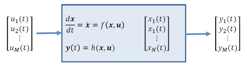
State-Space Representation

• State [𝒙]: A snapshot description of the system.

  (e. g. mobile robot location, robotic arm joint configuration)

• Input [𝒖]: What we can do to modify the state.

  (e. g. motor rotation)

• Output [𝒚]: What we can observe from the system.

  (e. g. readings from GPS, distance sensors, cameras, etc)

• Dynamics: How the state evolves over time (laws of physics)

Linear Time Invariant (LTI) systems

• Any system that can be represented in this shape is LTI:

$\dot{x}(t)=Ax(t)+Bu(t)$ $\dot{y}(t)=Cx(t)+Du(t)$ ​ Where 𝐴, 𝐵, 𝐶, 𝐷 are constant matrices/vectors.

• Linearity:
  • If input $u_1(𝑡)$produces output ${𝑦}_1(𝑡)$
  • and input ${𝑢}_2(𝑡)$ produces output ${𝑦}_2(𝑡)$
  • then input ${𝑎}_1{𝑢}_1(𝑡)+{𝑎}_2{𝑢}_2(𝑡)$ produces output ${𝑎}_1{𝑦}_1(𝑡)+{𝑎}_2{𝑦}_2(𝑡)$
• Time invariance
  • If input 𝑢(𝑡) produces output 𝑦(𝑡)
  • then input 𝑢(𝑡 − 𝑇) produces output 𝑦(𝑡 − 𝑇)

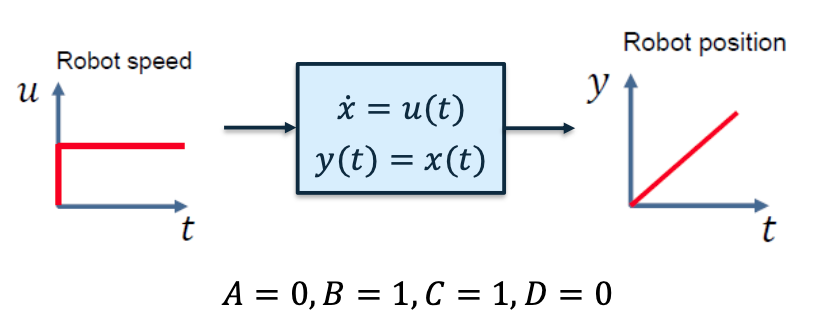
Single-Integrator System

Mobile robot with 1-dimensional motion

• State [𝑥]: robot position
• Input [𝑢]: robot speed
• Output [𝑦]: robot position

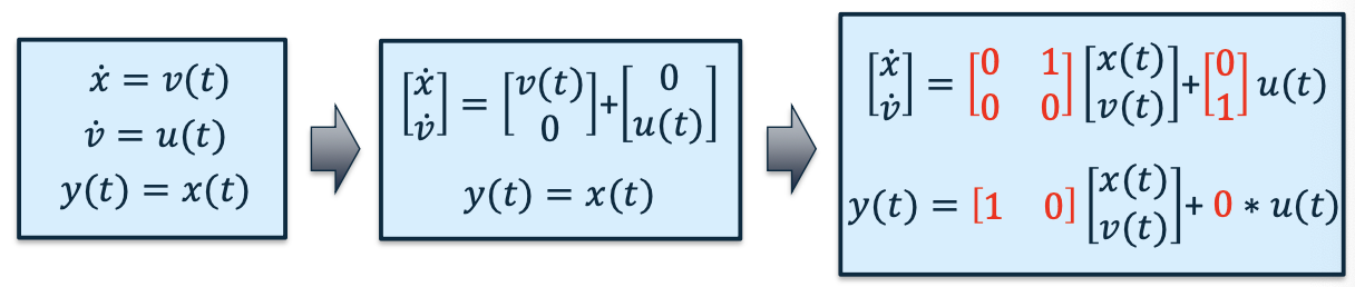
Double-Integrator System

Mobile robot with 1-dimensional motion

• State 1 [𝑥]: robot position
• State 2 [𝑣]: robot velocity
• Input [𝑢]: robot acceleration
• Output [𝑦]: robot position

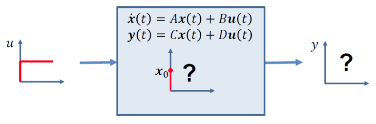
Output of the LTI System

Predict (or simulate) the dynamics of an LTI system

Given

• A LTI system with known 𝐴, 𝐵, 𝐶, 𝐷
• An initial state with ${𝑥}_0=𝑥(0)$
• A known input signal 𝑢(𝑡)

Find

• How state 𝑥 𝑡 and output 𝑦(𝑡)evolve over time

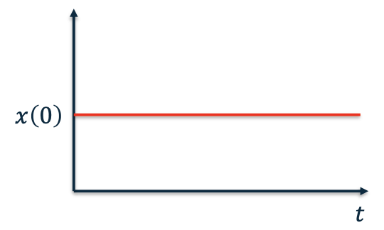
Initial Condition Response

• Consider no control input $\dot{x}=Ax$

• Now, if 𝐴 = 𝑎 is a scalar: $\dot{x}=ax$

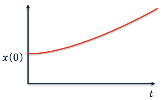
• The time response is given by

$$x(t)=e^{at}x(0)$$

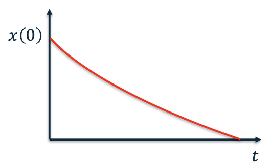
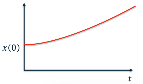
Exponential

• If a < 0
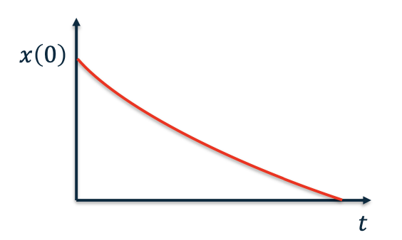
• If a > 0

Matrix Exponential

• Similarly, if 𝐴 is a matrix, the Taylor expansion of ${𝑒}^{𝐴}$ is
• Then we have
• Differentiating
• Hence, we have
• The time response is given by

Stability of the System

Lyapunov Stability

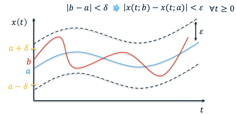
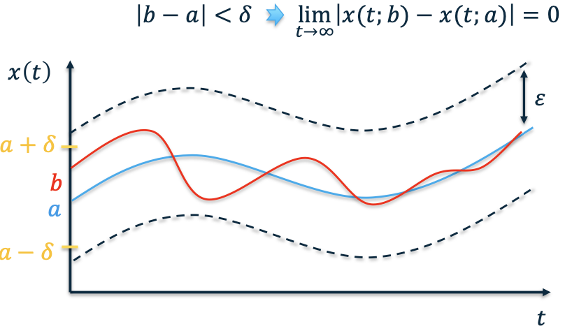
• Let 𝑥(𝑡; 𝑎) be a solution to $\dot{𝑥}=𝑓(𝑥)$ with initial condition 𝑎
• A solution is stable in the sense of Lyapunov if other solutions that start near 𝑎 stay close to $𝑥(𝑡;𝑎)$
• For all 𝜀 > 0 is there exists 𝛿 > 0 such that

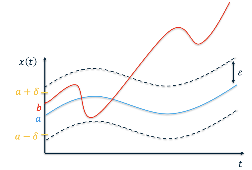
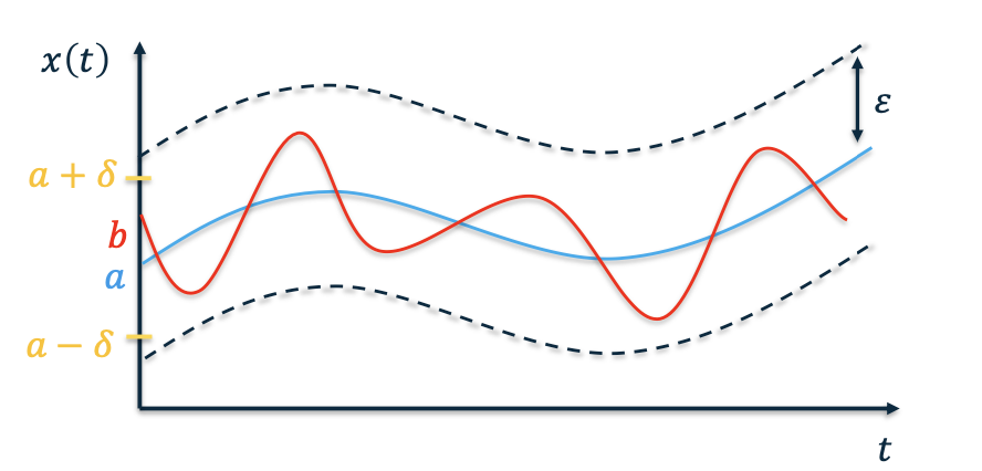
Unstable System

Asymptotic Stability

• When a system verifies the following:
  • It is Lyapunov stable
  • Additionally:

Neutral Stability

• When a system verifies the following:
  • It is Lyapunov stable
  • It is not asymptotically stable

Stability of the LTI System

$$\dot{𝑥}(t)=𝐴𝑥(t)+𝐵𝑢(𝑡)$$

• Let’s say $𝑢(t)$ is either known or depends on $𝑥(𝑡)$
• Can we determine the stability of the system from 𝐴, 𝐵 ?

Scalar Exponential Response

• Assuming no input, and 𝐴 is a scalar, we have

$$\dot{x}=axx(t)=e^{at}x(0)$$

• If 𝑎 < 0, the system is asymptotically stable

• If 𝑎 > 0, the system is not stable

• If 𝑎 = 0, the system is neutrally stable

Matrix Exponential Response

• If 𝐴 is a matrix, a matrix 𝐴 is diagonalisable if there is an invertible matrix 𝑇 and a diagonal matrix 𝛬 such that:

$$\mathrm{\Lambda }=T^{-1}AT=\left[\begin{array}{cccc}{\lambda }_1& 0& \cdots & 0\\ 0& {\lambda }_2& \cdots & 0\\ ⋮& ⋮& \ddots & ⋮\\ 0& 0& \cdots & {\lambda }_n\end{array}\right]$$

• Choose a set of coordinates 𝑧 for our state such that $Tz=x$

• Then $T\dot{z}=\dot{x}=Ax\dot{z}=T^{-1}ATz=\mathrm{\Lambda }z$

• $\dot{z}=\mathrm{\Lambda }\mathrm{z}$has the same stability properties as $\dot{𝑥}=𝐴𝑥$

$$A=\left[\begin{array}{cccc}{\lambda }_1& 0& \cdots & 0\\ 0& {\lambda }_2& \cdots & 0\\ ⋮& ⋮& \ddots & ⋮\\ 0& 0& \cdots & {\lambda }_n\end{array}\right]e^{\mathrm{\Lambda }t}=\left[\begin{array}{cccc}{e}^{{\lambda }_{1}t}& 0& \cdots & 0\\ 0& e^{{\lambda }_{2}t}& \cdots & 0\\ ⋮& ⋮& \ddots & ⋮\\ 0& 0& \cdots & e^{{\lambda }_{n}t}\end{array}\right]$$

• The system is asymptotically stable if ${\lambda }_i<0\mathrm{\forall }i\in \{1,2,...,n\}$

• The system is not stable if $\mathrm{\exists }{\lambda }_i>0i\in \{1,2,...,n\}$

• The system is neutrally stable if

$$\begin{gathered} \mathrm{\exists }{\lambda }_i=0i\in \{1,2,...,n\} \\ {\lambda }_i\le 0\mathrm{\forall }i\in \{1,2,...,n\} \end{gathered}$$

Example: Target Tracking

• The setup:

  • Given a mobile robots who can only measure the relative displacement of its target (no global coordinates)

  

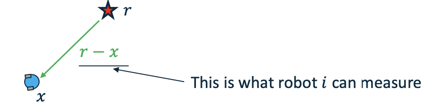
  • Problem: Have the robot meet at the desired position

• Robot dynamics: $\dot{x}=u$

• Controller design: $u=K(r-x)$

  r -> A positive constant

• Condition:

  • The target can always be detected by the robot using onboard/external sensors (e.g., a camera)

Theoretical guarantee

• Define tracking error signal $𝑒=𝑟-𝑥$, we have $\dot{e}=-\dot{x}=-u=-Ke$

• Hence, the error system is asymptotically stable

Stability of Nonlinear Systems

• We consider nonlinear time-invariant system $\dot{𝑥}=𝑓(𝑥)$
• A point ${𝑥}_{𝑒}$ is an equilibrium point of the system if $𝑓({𝑥}_{𝑒})=0$

The system is globally asymptotically stable if for every trajectory $𝑥(𝑡)$, we have $𝑥(𝑡)\to {𝑥}_{𝑒}$ as $𝑡\to \infty$

Positive Definite Functions

A function $𝑉$ is positive definite if

• $𝑉(𝑥)\ge 0$ for all 𝑥
• $𝑉(𝑥)=0$ if and only if $𝑥=0$
• $𝑉(𝑥)\to \infty$ as $𝑥\to \infty$

Example: $𝑉(𝑥)={𝑥}^{𝑇}𝑃𝑥$, with $𝑃={𝑃}^{𝑇}$, is positive definite if and only if $𝑃>0$.

Lyapunov Theory

Lyapunov theory is used to make conclusions about trajectories of a system $\dot{𝑥}=𝑓(𝑥)$ without finding the trajectories (i.e., solving the differential equation)

a typical Lyapunov theorem has the form:

• If there exists a function $𝑉(𝑥)$ that satisfies some conditions on

  $𝑉$ and $\dot{𝑉}$.

• Then trajectories of system satisfy some property

If such a function $𝑉$ exists we call it a Lyapunov function (that proves the property holds for the trajectories)

Lyapunov Stability Theorem

Suppose there is a function $𝑉$ such that

• $𝑉(𝑥)$ is positive definite
• $\dot{𝑉}(𝑥)<0$ for all $𝑥\ne 0$, $\dot{𝑉}(0)=0$

Then, every trajectory of $\dot{𝑥}=𝑓(𝑥)$ converges to zero as $𝑡\to \infty$ (i.e., the system is globally asymptotically stable)

Lecture Summary

• Feedback Systems
• Bang-Bang Control
• PID Control
• State-Space Representation
• Stability of the System