Robotics Mapping

Mapping

Objectives:

1. Probabilistic mapping
2. Definition of SLAM
3. Multi-robot systems
   • Rendezvous
   • Formation control

Mapping

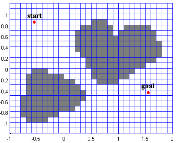
One of the vital, yet challenging, tasks for mobile robots is mapping an environment with unknown structure, where the robot needs to navigate and build a properly represented map.

Note that the robot has to move while building the map, and since the measurements are usually relative to the robot frame {𝑅}, transformation to the world frame {𝑊} requires an accurate knowledge of the robot pose.

The probabilistic methods for robotic mapping rely on studying the propagation of probabilistic distributions of the sensor noise and the unknown landmark locations.

One of these methods is occupancy grid mapping, which relies on Bayes’ theorem to recursively estimate the map as new measurements become available. 占用网格映射

Occupancy grid

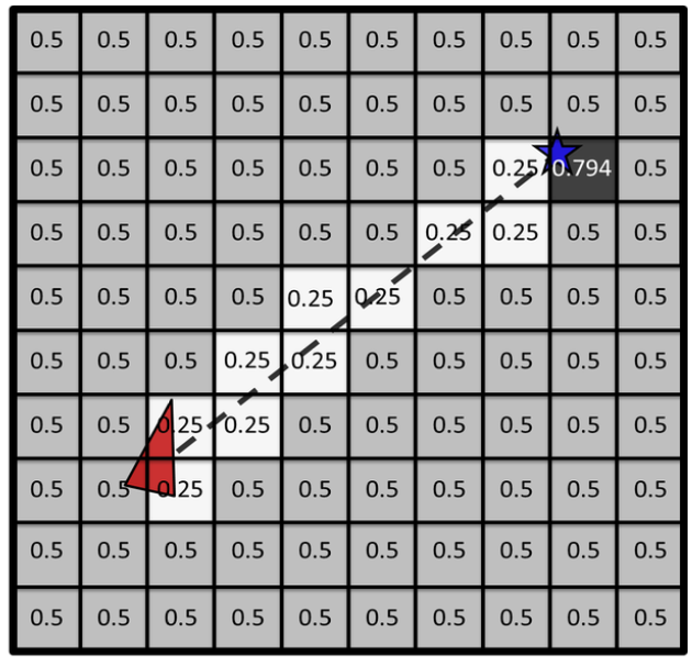
• In occupancy grid, the map is represented by a grid over the environment space, e.g., 2D or 3D space, and each cell of the grid corresponds to the probability of the cell being occupied. For example, in a deterministic world, empty cells are stored as ‘0’ and occupied cells as ‘1’.
• Of course, grids with high resolution result in more accurate maps, however, that comes at an expensive computational cost.

For a 2D space, each cell is denoted by $𝑐_{𝑖,𝑗} $where 𝑖 represents the 𝑥-axis index and 𝑗 represent the 𝑦-axis index. This grid can be represented by a matrix flipped vertically, where 𝑖 corresponds to the column, and 𝑗 corresponds to the row.

Binary mapping

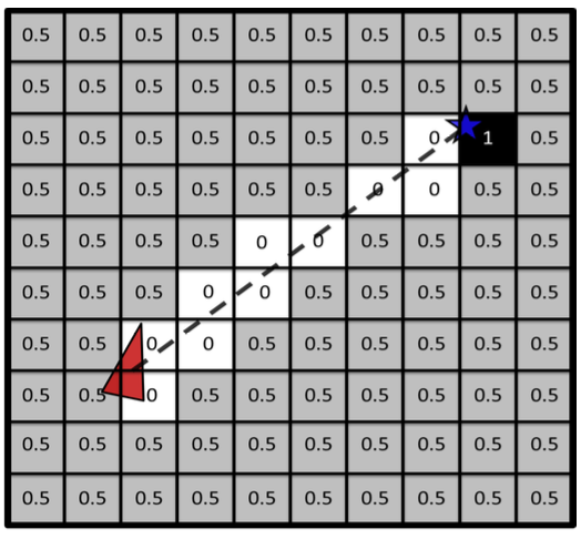
• If the probability is 100%, $𝑐_{i,j} = 1$.

• If it is unknown, it is usually set to $𝑐_{i,j} = 0.5$.

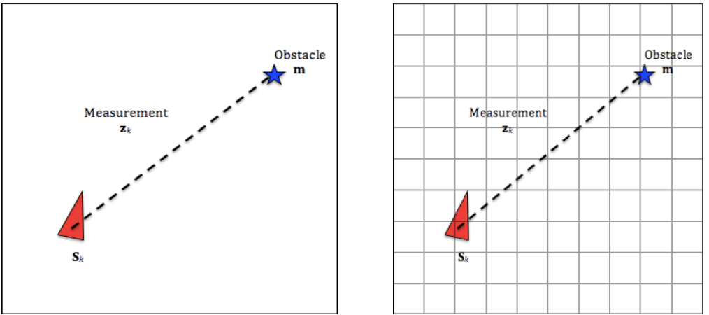
• In order to compute the obstacle position 𝐦, the measurement $z_𝑘$ and the robot pose $s_k$ are used as follows:

\[m_{x}=s_{x,k}+z_{\rho,k}\cos(s_{\theta,k}+z_{\alpha,k})\] \[m_{y}=s_{y,k}+z_{\rho,k}\sin(s_{\theta,k}+z_{\alpha,k})\]

Probabilistic mapping

• Based on Sensor Probabilistic Model

Discrete Random Variables

Let’s define 𝑋 as a random variable.

If this variable is discrete, then $𝑃 (𝑋 = 𝑥)$ is the probability that the R.V., 𝑋, will take the value 𝑥.

Formally, $𝑝 (𝑥) = 𝑃(𝑋 = 𝑥)$ is known as the probability mass function. \(\sum_{i=1}^\infty p(x_i)=1\)

Dice Example 🎲

$ \operatorname {Let}X={1,2,3,4,5,6}$

\[p(1)=p(2)=p(3)=p(4)=p(5)=p(6)=\frac16\] \[p(odd)=p(1)+p(3)+p(5)=\frac12\]

Joint Distribution

Now let’s have two R.V., 𝑋 and 𝑌. \(𝑝 (𝑥, 𝑦) = 𝑝 (𝑋 = 𝑥 \ 𝑎𝑛𝑑 \ 𝑌 = 𝑦)\) If 𝑋 and 𝑌 are independent, i.e. knowing the value of one of them does not change the distribution of the other, then \(𝑝 (𝑥, 𝑦) = 𝑝 (𝑥) 𝑝(𝑦)\)

Conditional Probability

If two R.V. are related, i.e. knowledge of one influences the distribution of the other. \(p(x|y)=p(X=x\text{ knowing that }Y=y)\)

\[p(x|y)=\frac{p(x,y)}{p(y)}\]

If X and Y are independent, \(p(x|y)=\frac{p(x,y)}{p(y)}=p(x)\)

Bayes Rule

The Bayes Rule relates the conditional probability of two random variable to its inverse and is used in many localisation filtering algorithms (Markov and Kalman for example). \(p(x|y)=\frac{p(y|x)p(x)}{p(y)}\)

Probabilistic Mapping 概率映射

• Let 𝑍 be a continuous random variable that corresponds to the true distance between the robot and the obstacle, and let $c_{i,j}$ be a discrete random variable that corresponds to the $𝑖𝑗$ cell in the grid being empty or occupied.

• Taking into account the nature of the LiDAR where it uses the line-of-sight principle, there are two possible events for each measurement: (i) $𝑍 = 𝑧_𝑘$ , or (ii) $𝑍 < 𝑧_𝑘$ . Moreover, since $c_{i,j}$ is discrete random variable, there are only two possible events for the cell: (i) $c_{i,j} = 𝑜𝑐𝑐𝑢𝑝𝑖𝑒𝑑$, or (ii) $c_{i,j} ≠ 𝑜𝑐𝑐𝑢𝑝𝑖𝑒𝑑$.
• Sensor model – four different probabilities

Sensor Characteristics

1) The probability of correctly detecting the obstacle given that there is an obstacle at $c_{i,j}$ This sensor characteristic is named sensor true positive. This is a measure of ‘how good’ the sensor is.

\[\Pr(Z=z_k\mid c_{i,j}=occupied)\]

2) Probability of correctly detecting free space given that the cell $c_{i,j}$ is not occupied. This sensor characteristic is named sensor true negative. This is also a measure of ‘how good’ the sensor is.

\[\Pr(Z<z_k\mid c_{i,j}\neq occupied)\]

3) Probability of detecting an obstacle at $c_{i,j}$ given there is no obstacle. This sensor characteristic is named sensor false positive. Because the sensor can also do mistakes, this is a measure of ‘how bad’ the sensor is.

\[\Pr(Z=z_k\mid c_{i,j}\neq occupied)\]

4) Probability of detecting free space given that there is obstacle at cell $c_{i,j}$. This sensor characteristic is named sensor false negative. This is also a measure of ‘how bad’ the sensor is.

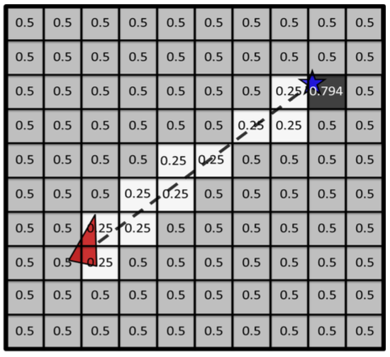
\[\Pr(Z<z_k\mid c_{i,j}= occupied)\]

Probabilistic Occupancy

Using Bayes’ theorem: \(P_r(A|B)=\frac{P_r(B|A)P_r(A)}{P_r(B)}\) where the event A is related to the probability of the cell of being occupied, and the event B is the probability related to the measurement from the sensor.

Probabilistic Mapping 重点

• Computing $\Pr(c_{i,j}=occupied

  Z=z_k)$

\[\Pr(c_{i,j}=occupied|Z=z_k)=\frac{\Pr(Z=z_k|c_{i,j}=occupied)\cdot\Pr(c_{i,j}=occupied)}{\Pr(Z=z_k)}\]

The law of total probability for two events A and B is: \(P_r(B)=P_r(B|A)P_r(A)+P_r(B|A)P_r(\bar{A})\)

\[P_{r}(Z=z_{k})=P_{r}\left(Z=z_{k}|c_{i,j}=occupied\right)\cdot P_{r}(c_{i,j}=occupied)+P_{r}\left(Z=z_{k}|c_{i,j}\neq occupied\right)\cdot P_{r}(c_{i,j}\neq occupied)\]

• Numerical values

\[\begin{aligned} & P_{r}(c_{i,j}=occupied)=0.5\quad\leftarrow prior\ probability \\ & P_{r}(Z=z_{k}|c_{i,j}=occupied)=0.85\leftarrow sensor\ true\ positive \\ & P_{r}(Z=z_{k}|c_{i,j}\neq occupied)=0.22\leftarrow sensor\ false\ positive \end{aligned}\] \[\begin{aligned} P_{r}(Z=z_{k}) & =P_{r}\left(Z=z_{k}|c_{i,j}=occupied\right)\cdot P_{r}(c_{i,j}=occupied) \\ & +P_{r}\left(Z=z_{k}|c_{i,j}\neq occupied\right)\cdot(1-P_{r}(c_{i,j}=occupied)) \end{aligned}\] \[P_r(Z=z_k)=(0.85*0.5)+(0.22*0.5)=0.425+0.11=0.535\]

• Posterior probability:

\[P_r(c_{i,j}=occupied|Z=z_k)=\frac{0.85*0.5}{0.535}=\frac{0.425}{0.535}=0.794\]

The probability of the cell occupancy after incorporating the measurement $𝑧_𝑘$

==要会算==

Autonomous Robots

The ultimate goal of an autonomous mobile robot is to move around an unknown or dynamic environment without any human intervention.

To be able to do this, the robot needs to be able to build up a map of the environment and localise itself within it.

The process of doing this is known as Simultaneous Localisation And Mapping or SLAM.

SLAM Definition(不考)

SLAM is the process of constructing a map of the environment based on knowledge of the path of the robot and measurements of the surrounding area.

The process is limited to only using sensors on the robot itself, either proprioceptive (odometry) or exteroceptive (laser scanners).

Given input readings from odometry, 𝑈𝑇, and environmental sensor readings, 𝑍𝑇, SLAM is the process of recovering the robot path, 𝑋𝑇, and the map of the environment, 𝑀𝑇.

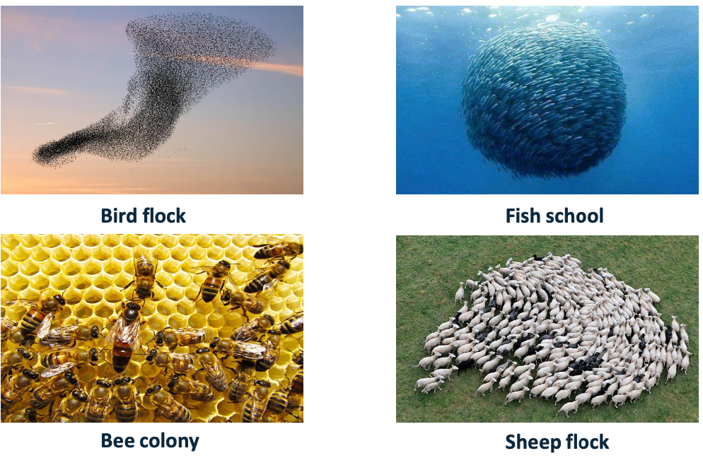
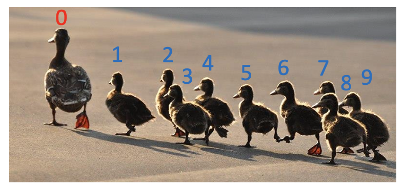
Collective Movements in Nature

Multi-Robot Systems

• Definition:
  • A system consisted of multiple robots which can cooperate with each other to achieve a common goal.

Centralized vs Distributed

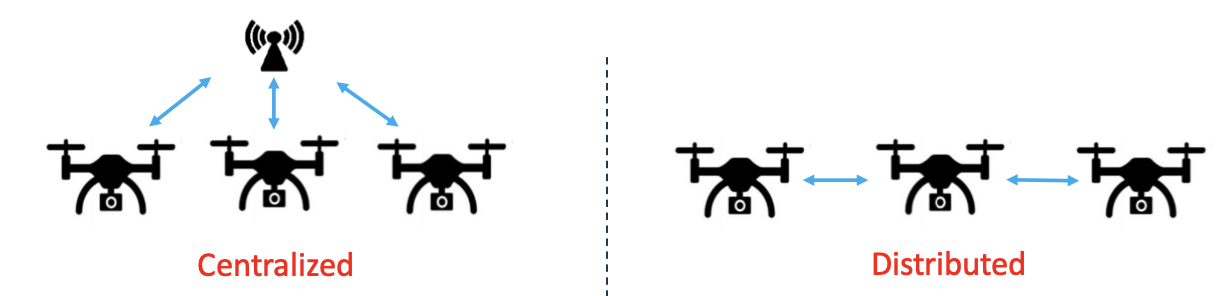
Centralized

• One control unit communicates with all robots to issue commands

• Require synchronized and

reliable communication channels

• Suffer from single-point failures

Distributed

• Each robot only needs to communicate with its neighbors

• Scalable and robust to failure

• Reduce the bandwidth requirement

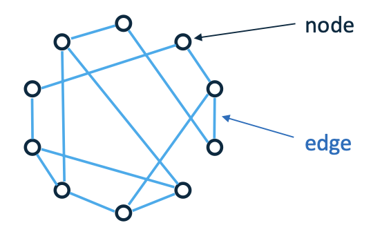
Communication Topologies

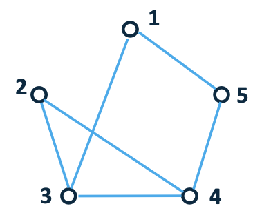
• Basic graph theory

  • An edge rooted at the $𝑗^{𝑡ℎ}$ node and ended at the $𝑖_{𝑡ℎ}$node is denoted by 𝑗, 𝑖 , which means information can flow from node 𝑖 to node 𝑗. $𝑎_{𝑖𝑗} =1$ is the weight of edge 𝑗, 𝑖 .

    

  • Example:

    

\[\begin{aligned} & a_{12}=a_{21}=\quad0\quad a_{13}=a_{31}=\quad1\quad a_{14}=a_{41}=\quad0\quad a_{15}=a_{51}=\quad1 \\ & a_{23}=a_{32}=\quad1\quad a_{24}=a_{42}=\quad1\quad a_{25}=a_{52}=\quad1 \\ & a_{34}=a_{43}=\quad1\quad a_{35}=a_{53}=\quad0 \\ & a_{45}=a_{54}=\quad1 \end{aligned}\]

Rendezvous of Multiple Robots

• The setup:

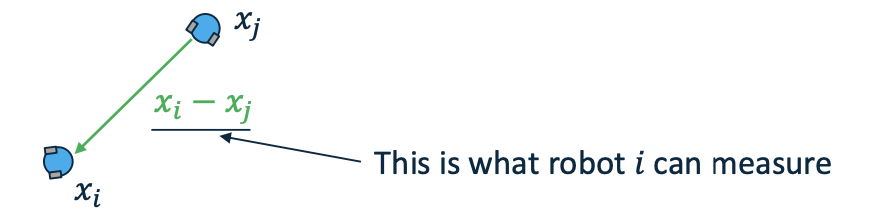
  • Given a collection of mobile robots who can only measure the relative displacement of their neighbors (no global coordinates)

    

  • Problem: Have all the robots meet at the same position

• Robot dynamics: $\dot{x}_i=u_i$
• Rendezvous control protocol design: $u_i=-K\sum_{j=1}^Na_{ij}(x_i-x_j)$
• Assumption:
  • The communication graph among all the robots is connected.

Extension to Formation Control

Formation control is a coordinated control for a fleet of robots to follow a predefined trajectory while maintaining a desired spatial pattern.

• Leader-follower mechanism:

  

• Formation control protocol design: $u_i=-K\sum_{j=0}^Na_{ij}[(x_i-h_i)-(x_j-h_j)]$

Example: \(\begin{aligned} & h_{1}= \begin{bmatrix} -2 \\ -2 \\ 2 \end{bmatrix} & h_{2}= \begin{bmatrix} 2 \\ -2 \\ 2 \end{bmatrix} \\ & h_{3}= \begin{bmatrix} -2 \\ 2 \\ 2 \end{bmatrix} & h_{4}= \begin{bmatrix} 2 \\ 2 \\ 2 \end{bmatrix} \\ & h_{5}= \begin{bmatrix} -2 \\ -2 \\ -2 \end{bmatrix} & h_{6}= \begin{bmatrix} 2 \\ -2 \\ -2 \end{bmatrix} \\ & h_{7}= \begin{bmatrix} -2 \\ 2 \\ -2 \end{bmatrix} & h_{8}= \begin{bmatrix} 2 \\ 2 \\ -2 \end{bmatrix} \end{aligned}\)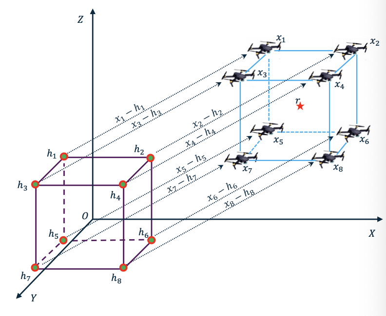

…