2025-09-23-Supervised Machine Learning Lecture 4 Model selection

Supervised Machine Learning Lecture 4 Model selection

Model selection and Occam’s Razor

• Occam’s razor principle “Entities should not be multiplied unnecessarily” captures the trade-off between generalization error and complexity
• Model selection in machine learning can be seen to implement Occam’s razor

Stochastic scenario

• The analysis so far assumed that the labels are deterministic functions of the input
• Stochastic scenario relaxes this assumption by assuming the output is a probabilistic function of the input
• The input and output is generated by a joint probability distribution $D$ or $X \times \mathcal{Y}$.
• This setup covers different cases when the same input $x$ can have different labels $y$
• In the stochastic scenario, there may not always exist a target concept $f$ that has zero generalization error $R(f) = 0$

Sources of stochasticity

The stochastic dependency between input and output can arise from various sources

• Imprecision in recording the input data (e.g. measurement error), shifting our examples in the input space
• Errors in the labeling of the training data (e.g. human annotation errors), flipping the labels some examples
• There may be additional variables that affect the labels that are not part of our input data

All of these sources could be characterized as adding noise (or hiding signal)

Noise and complexity

• The effect of noise is typically to make the decision boundary more complex
• To obtain a consistent hypothesis on noisy data, we can use a more complex model e.g. a spline curve instead of a hyperplane
• But this may not give a better generalization error, if we end up merely re-classifying points corrupted by noise

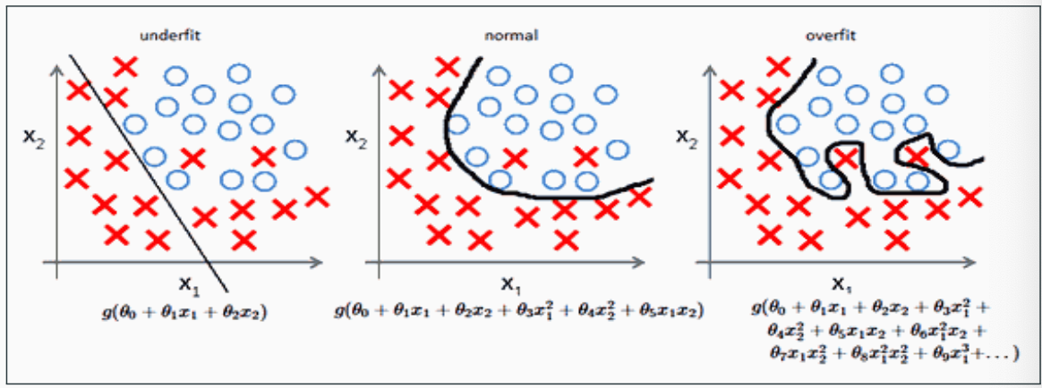
In practice, we need to balance the complexity of the hypothesis and the empirical error carefully

• A too simple model does not allow optimal empirical error to obtained, this is called underfitting
• A too complex model may obtain zero empirical error, but have worse than optimal generalization error, this is called overfitting

Controlling complexity

Two general approaches to control the complexity

• Selecting a hypothesis class, e.g. the maximum degree of polynomial to fit the regression model
• Regularization: penalizing the use of too many parameters, e.g. by bounding the norm of the weights (used in SVMs and neural networks)

  Measuring complexity

What is a good measure of complexity of a hypothesis class?

We have already looked at some measures:

• Number of distinct hypotheses $

  \mathcal{H}

  $: works for finite $\mathcal{H}$ (e.g. models build form binary data), but not for infinite classes (e.g. geometric hypotheses such as polygons, hyperplanes, ellipsoids)

• Vapnik-Chervonenkis dimension (VCdim): the maximum number of examples that can be classified in all possible ways by choosing different hypotheses $h \in \mathcal{H}$
• Rademacher complexity: measures the capability to classify after randomizing the labels

Lots of other complexity measures and model selection methods exist c.f. https://en.wikipedia.org/wiki/Model_selection (these are not in the scope of this course)

Bayes error

Bayes error

• In the stochastic scenario, there is a minimal non-zero error for any hypothesis, called the Bayes error
• Bayes error is the minimum achievable error, given a distribution $D$ over $X \times \mathcal{Y}$, by measurable functions $h : X \mapsto \mathcal{Y}$

\[R^* = \inf_{\{h|h \text{ measurable }\}} R(h)\]

• Note that we cannot actually compute $R^*$:
  • We cannot compute the generalization error $R(h)$ exactly (c.f. PAC learning)
  • We cannot evaluate all measurable functions (intuitively: hypothesis class that contains all functions that are mathematically well-behaved enough to allow us to define probabilities on them)
• Bayes error serves us a a theoretical measure of best possible performance

Bayes error and noise

• A hypothesis with $R(h) = R^{*}$ is called the Bayes classifier
• The Bayes classifier can be defined in terms of conditional probabilities as

\[h_{Bayes}(x) = \arg\max_{y \in \{0, 1\}} Pr(y|x)\]

• The average error made by the Bayes classifier at $x \in X$ is called the noise

\[noise(x) = \min(Pr(1|x), Pr(0|x))\]

• Its expectation $E(noise(x)) = R^{*}$ is the Bayes error
• Similarly to the Bayer error, Bayes classifier is a theoretical tool, not something we can compute in practice

Bayes error example

• We have a univariate input space:
  $x \in {1, 2, 3}$, and two classes
  $y \in {0, 1}$.
• We assume a uniform distribution of data:
  $Pr(x) = 1/3$
• The Bayes classifier will predict the most probable class for each possible input value

| $X$ | 1 | 2 | 3 | |———|—–|—–|—–| | $P(Y=1|X)$| 0.6 | 0.2 | 0.7 | | $P(Y=0|X)$ | 0.4 | 0.8 | 0.3 | | $h_{Bayes}(x)$ | 1 | 0 | 1 | | $noise(x)$ | 0.4 | 0.2 | 0.3 |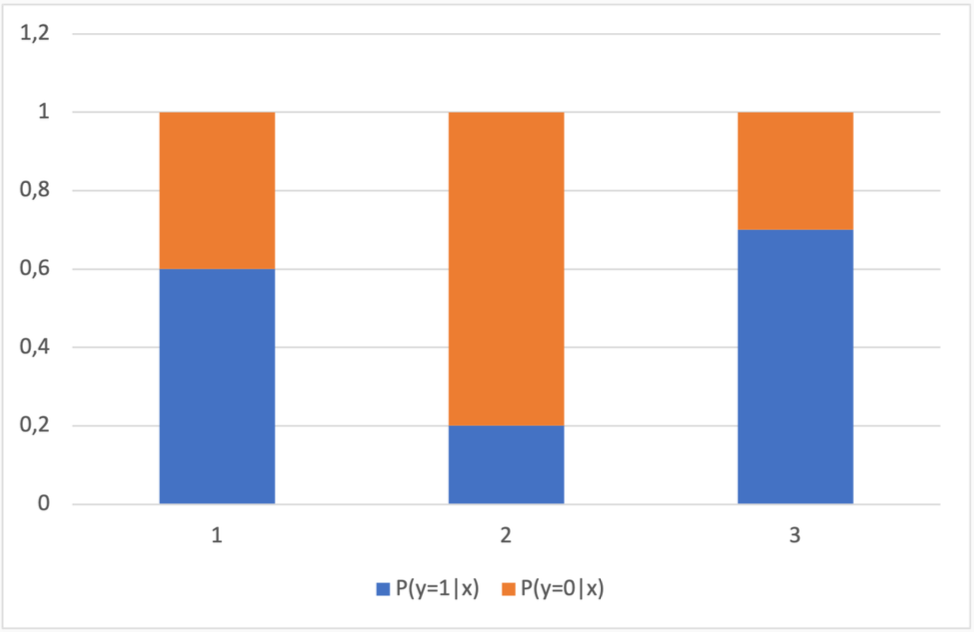

The Bayes error is the expectation of the the noise over the input domain

\[R^* = \sum_x P(x) noise(x) = \frac{1}{3}(0.4 + 0.2 + 0.3) = 0.3\]

Decomposing the error of a hypothesis

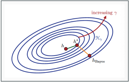
The excess error of a hypothesis compared to the Bayes error $R^*$ can be decomposed as:

\[R(h) - R^* = \epsilon_{estimation} + \epsilon_{approximation}\]

• $\epsilon_{estimation} = R(h) - R(h^)$ is the excess generalization error $h$ has over the optimal hypothesis $h^ = \arg\min_{h’ \in \mathcal{H}} R(h’)$ in the hypothesis class $\mathcal{H}$
• $\epsilon_{approximation} = R(h^) - R^$ is the approximation error due to selecting the hypothesis class $\mathcal{H}$ instead of the best possible hypothesis class (which is generally unknown to us)

Note: The approximation error is sometimes called the bias and the estimation error the variance, and the decomposition bias-variance decomposition

Figure on the right depicts the concepts: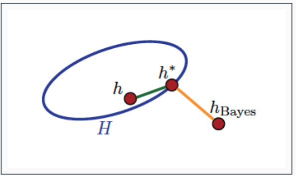

• $h_{Bayes}$ is the Bayes classifier, with
  $R(h_{Bayes}) = R^*$
• $h_* = \inf_{h \in \mathcal{H}} R(h)$ is the hypothesis with the lowest generalization error in the hypothesis class $\mathcal{H}$
• $h$ has both non-zero estimation error
  $R(h) - R(h^)$ and approximation error
  $R(h^) - R(h_{Bayes})$

Example: Approximation error

• Assume the hypothesis class of univariate threshold functions:

  \[\mathcal{H} = \{ h_{a,\theta} : X \mapsto \{0,1\} \mid a \in \{-1,+1\}, \theta \in \mathbb{R} \},\]

  where $h_{a,\theta}(x) = \mathbf{1}_{ax \geq \theta}$

• The classifier from $\mathcal{H}$ with the lowest generalization error separates the data with $x=3$ from data with $x < 3$ by, e.g. choosing $a=1, \theta=2.5$, giving $h^(1) = h^(2) = 0, h^*(3) = 1$

  \[\begin{array}{c|ccc} X & 1 & 2 & 3 \\ \hline P(y=1|x) & 0.6 & 0.2 & 0.7 \\ P(y=0|x) & 0.4 & 0.8 & 0.3 \\ h^*(x) & 0 & 0 & 1 \\ \end{array}\]

• The generalization error is \(R(h^*) = \frac{1}{3}(0.6 + 0.2 + 0.3) \approx 0.367\)

• Approximation error satisfies:

  \[\epsilon_{\text{approximation}} = R(h^*) - R^* \approx 0.367 - 0.3 \approx 0.067\]

Example: estimation error

• Consider now a training set on the right consisting of $m = 13$ examples from the same distribution as before

  \[\begin{array}{c|ccc} x & 1 & 2 & 3 \\ \hline y=1 & 3 & 1 & 3 \\ y=0 & 1 & 3 & 2 \\ \hline \sum & 4 & 4 & 5 \end{array}\]

• The classifier from $h \in \mathcal{H}$ with the lowest training error $\hat{R}(h) = 0.385$ separates the data with $x = 1$ from data with $x > 1$ by, e.g. choosing $a = -1, \theta = 1.5$, giving $h(1) = 1, h(2) = h(3) = 0$

• However, the generalization error of $h$ is \(R(h) = \frac{1}{3} \left(0.4 + 0.2 + 0.7\right) \approx 0.433\)

• The estimation error satisfies \(\epsilon_{estimation} = R(h) - R(h^*) \approx 0.433 - 0.367 \approx 0.067\)

• The decomposition of the error of h is given by: \(R(h) = R^* + \epsilon_{approximation} + \epsilon_{estimation} \approx 0.3 + 0.067 + 0.067 \approx 0.433\)

Error decomposition and model selection

• We can bound the estimation error $\epsilon_{estimation} = R(h) - R(h^*)$ by generalization bounds arising from the PAC theory
• However, we cannot do the same for the approximation error since $\epsilon_{approximation} = R(h^) - R^$ remains unknown to us
• In other words, we do not know how good the hypothesis class is for approximating the label distribution

Complexity and model selection

In model selection, we have a trade-off: increasing the complexity of the hypothesis class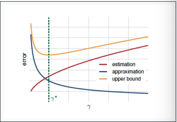

• decreases the approximation error as the class is more likely to contain a hypothesis with error close to the Bayes error

• increases the estimation error as finding the good hypothesis becomes more hard and the generalization bounds become looser (due to increasing $\log

  \mathcal{H}

  $ or the VC dimension)

To minimize the generalization error over all hypothesis classes, we should find a balance between the two terms

Learning with complex hypothesis classes

• One strategy for model selection to initially choose a very complex hypothesis class with zero or very low empirical risk $\mathcal{H}$
• Assume in addition the class can be decomposed into a union of increasingly complex hypothesis classes $\mathcal{H} = \bigcup_{\gamma \in \Gamma} \mathcal{H}_{\gamma}$, parametrized by $\gamma$, e.g.
  • $\gamma =$ number of variables in a boolean monomial
  • $\gamma =$ degree of a polynomial function
  • $\gamma =$ size of a neural network
  • $\gamma =$ regularization parameter penalizing large weights
• We expect the approximation error to go down and the estimation error to up when $\gamma$ increases
• Model selection entails choosing $\gamma^{*}$ that gives the best trade-off

Half-time poll: Inequalities on different errors

Let $R_*$ denote the Bayes error, $R(h)$ the generalization error and $\hat{R}_S(h)$ the training error of hypothesis $h$ on training set $S$.

Which of the inequalities always hold true?

1. $R^* \leq \hat{R}_S(h)$
2. $\hat{R}_S(h) \leq R(h)$
3. $R^* \leq R(h)$

Answer to the poll in Mycourses by 11:15: Go to Lectures page and scroll down to “Lecture 4 poll”:

Answers are anonymous and do not affect grading of the course.

Regularization-based algorithms

Regularization-based algorithms

• Regularization is technique that penalizes large weights in a model based on weighting input features:
  • linear regression, support vector machines and neural networks are fall under this category
• An important example is the class of linear functions $x ↦ 𝗐ᵀ𝗑$
• The classes as parametrized by the norm $‖w‖$ of the weight vector bounded by $γ: H₍γ₎ = {x ↦ 𝗐ᵀ𝗑 : ‖\mathbf w‖ ≤ γ}$
• The norm is typically either
  • $L²$ norm (Also called Euclidean norm or 2-norm):
    $‖\mathbf w‖₂ = √∑ⱼ₌₁ⁿ wⱼ²$: used e.g. in support vector machines and ridge regression
  • $L$¹ norm (Also called Manhattan norm or 1-norm):
    $‖\mathbf w‖₁ = ∑ⱼ₌₁ⁿ |wⱼ|$: used e.g. in LASSO regression

Regularization-based algorithms

• For the $L^{2}$-norm case, we have an important computational shortcut: the empirical Rademacher complexity of this class can be bounded analytically!
• Let $S \subset {\mathbf{x} \mid |\mathbf{x}| \leq r}$ be a sample of size $m$ and let \(\mathcal{H}_{\gamma} = \{\mathbf{x} \mapsto \mathbf{w}^{T}\mathbf{x} : \|\mathbf{w}\|_{2} \leq \gamma\} \text{. Then}\) \(\hat{\mathcal{R}}_{S}(\mathcal{H}_{\gamma}) \leq \sqrt{\frac{r^{2} \gamma^{2}}{m}} = \frac{r\gamma}{\sqrt{m}}\)
• Thus the Rademacher complexity depends linearly on the upper bound $\gamma$ norm of the weight vector, as $r$ and $m$ are constant for any fixed training set

• We can use $|\mathbf{w}|$ as a efficiently computable upper bound of $\hat{\mathcal{R}}{m}(\mathcal{H}{\gamma})$

• A regularized learning problem is to minimize
  \(\arg\min_{h \in \mathcal{H}} \hat{R}_S(h) + \lambda \Omega(h)\)

• $\hat{R}_S(h)$ is the empirical error
• $\Omega(h)$ is the regularization term which increases when the complexity of the hypothesis class increases
• $\lambda$ is a regularization parameter, which is usually set by cross-validation
• For the linear functions $h : \mathbf{x} \mapsto \mathbf{w}^T \mathbf{x}$, usually $\Omega(h) = |\mathbf{w}|_2^2$ or $\Omega(h) = |\mathbf{w}|_1$
• We will study regularization-based algorithms during the next part of the course

Model selection using a validation set

Model selection by using a validation set

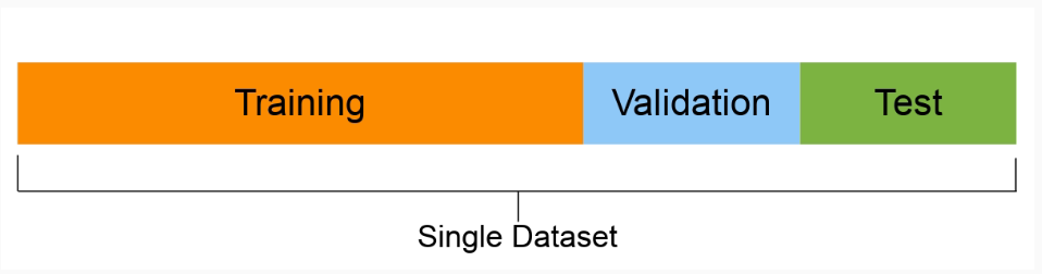
We can use the given dataset for empirical model selection, if the algorithm has input parameters (hyperparameters) that define/affect the model complexity

• Split the data into training, validation and test sets
• For the hyperparameters, use grid search to find the parameter combination that gives the best performance on the validation set
• Retrain a final model using the optimal parameter combination, use both the training and validation data for training
• Evaluate the performance of the final model on the test set

Grid search

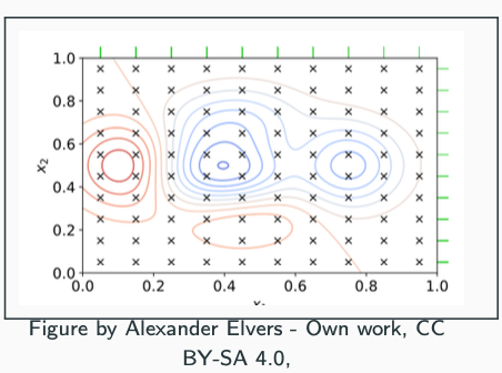
• Grid search is an technique frequently used to optimize hyperparameters, including those that define the complexity of the models
• In its basic form it goes through all combinations of parameter values, given a set of candidate values for each parameter
• For two parameters, taking of value combinations $(v, u) \in V \times U$, where $V$ and $U$ are the sets of values for the two parameters, defines a two-dimensional grid to be searched
• Even more parameters can be optimized but the exhaustive search becomes computationally hard due to exponentially exploding search space

Model selection by using a validation set

• The need for the validation set comes from the need to avoid overfitting
• If we only use a simple training/test split and selected the hyperparameter values by repeated evaluation on the test set, the performance estimate will be optimistic
• A reliable performance estimate can only be obtained form the test set

How large should the training set be in comparison of the validation set?

• The larger the training set, the better the generalization error will be (e.g. by PAC theory)
• The larger the validation set, the less variance there is in the test error estimate.
• When the dataset is small generally the training set is taken to be as large as possible, typically 90% or more of the total
• When the dataset is large, training set size is often taken as big as the computational resources allow

Stratification

• Class distributions of the training and validation sets should be as similar to each another as possible, otherwise there will be extra unwanted variance
  • when the data contains classes with very low number of examples, random splitting might result in no examples in the class in the validation set
• Stratification is a process that tries to ensure similar class distributions across the different sets
• Simple stratification approach is to divide all classes separately into the training and validation sets and the merge the class-specific training sets into global training set and class-specific validation sets into a global validation set.

Cross-validation

The need of multiple data splits

One split of data into training, validation and test sets may not be enough, due to randomness:

• The training and validation sets might be small and contain noise or outliers
• There might be some randomness in the training procedure (e.g. initialization)
• We need to fight the randomness by averaging the evaluation measure over multiple (training, validation) splits
  • The best hyperparameter values are chosen as those that have the best average performance over the n validation sets.

Generating multiple data splits

• Let us first consider generating a number of training and validation set pairs, after first setting aside a separate test set
• Given a dataset $S$, we would like to generate $n$ random splits into training and validation set
• Two general approaches:
  • Repeated random splitting
  • n-fold cross-validation

n-Fold Cross-Validation

• The dataset S is split randomly into n equal-sized parts (or folds)

• We keep one of the n folds as the validation set (light blue in the Figure) and combine the remaining n - 1 folds to form the training set for the split
  

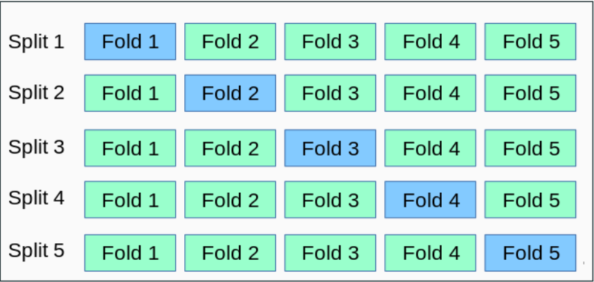
• n = 5 or n = 10 are typical numbers used in practice

Leave-one-out cross-validation (LOO)

• Extreme case of cross-validation is leave-one-out (LOO) : given a dataset of m examples, only one example is left out as the validation set and training uses the m − 1 examples.
• This gives an unbiased estimate of the average generalization error over samples of size m − 1 (Mohri, et al. 2018, Theorem 5.4.)
• However, it is comptationally demanding to compute if m is large

Nested cross-validation

• n-fold cross-validation gives us a well-founded way for model selection
• However, only using a single test set may result in unwanted variation
• Nested cross-validation solves this problem by using two cross-validation loops

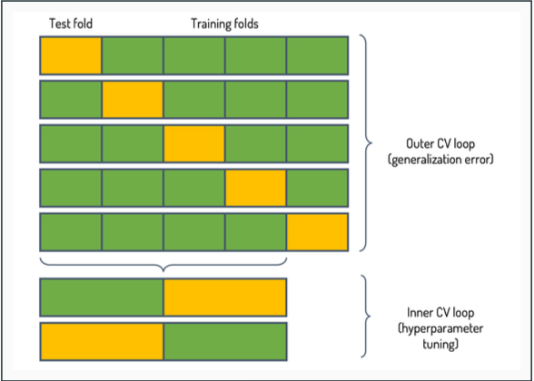
The dataset is initially divided into n outer folds (n = 5 in the figure)

• Outer loop uses 1 fold at a time as a test set, and the rest of the data is used in the inner fold
• Inner loop splits the remaining examples into k folds, 1 fold for validation, k−1 for training (k = 2 in the figure)

The average performance over the n test sets is computed as the final performance estimate

Summary

• Model selection concerns the trade-off between model complexity and empirical error on training data
• Regularization-based methods are based on continuous parametrization the complexity of the hypothesis classes
• Empirical model selection can be achieved by grid search on a validation dataset
• Various cross-validation schemes can be used to tackle the variance of the performance estimates