UL Lecture 2
UL Lecture 2 Part 2: Density estimation
Literature
CHACÓN, J. & DUONG, T. (2018) [C]
Multivariate kernel smoothing and its application. CRC Press. Sec 2.1-2.2, 3.1HASTIE, T., TIBSHIRANI, R., & FRIEDMAN, J. (2001) [H]
The Elements of Statistical Learning. Springer. Sec 6.8, 7.6-7.7, 8.5MURPHY, K.P. (2012) [M]
Machine Learning: A Probabilistic Perspective. The MIT Press. Section 11.2-11.5, 14.7
Overview of Part 2
We will…
- introduce mixture models as a parametric device for density estimation;
- elaborate, in detail, on the concept and implementation of the EM algorithm for the estimation of finite Gaussian mixtures;
- discuss the choice of the number of components as well as variance parameterizations;
- starting from histograms, introduce the concept of kernel density estimation;
- discuss the question of bandwidth selection;
- in either case, illustrate how to visualize the estimated densities.
Density estimation
Density estimation is the process of estimating the density ( f ) from data whose distribution the density is supposed to describe. We distinguish two families of methods:
Parametric density estimation. Here we use a flexible but finite-dimensional set of distributions to model the density, coordinated by a set of parameters, and the task is to estimate the parameters of the model. The model that we are going to use is a mixture model.
Nonparametric density estimation. Here we use an infinite-dimensional set of distributions to model the density, constrained only to have a certain degree of smoothness. We are going to use kernel smoothing for this purpose.
Mixture models
We take the view that the data consist of several subpopulations. We say the population is heterogeneous.
We do not know to which subpopulation an item (observation) belongs. Statisticians refer to this situation as unobserved heterogeneity.
We do assume, however, that each subpopulation can be described by a parametric distribution (such as Gaussian), which is known up to some parameters.
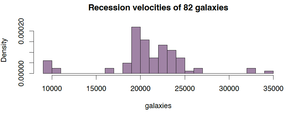
Example (1): Recession velocities in km/sec of 82 galaxies of an unfilled survey of the Corona Borealis region. Multimodality in such surveys is evidence for voids and superclusters in the far universe.
Data with unobserved heterogeneity
1
2
3
data(galaxies, package="MASS")
hist(galaxies, freq=FALSE, breaks=18, col="#68246d90",
     main="Recession velocities of 82 galaxies")
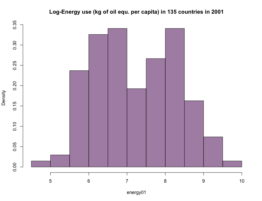
Example (2): Energy use data
1
2
3
4
5
6
7
energy.use <read.csv("http://www.maths.dur.ac.uk/~dma0je/Data/energy.csv", header=TRUE)

energy01 <log(energy.use[,c("X2001")])

hist(energy01,
     main="Log-Energy use\n(kg of oil equ. per capita)\nin 135 countries in 2001",
     freq=FALSE)
Aim: Fit ‘mixture’ distribution
We need to estimate the mixture ‘centres’, standard deviations, and proportions.
Gaussian mixture models
Data set $Y = { y_i \in \mathbb{R} }_{i \in [1..n]}$, independent given parameters $\theta$.
Unobserved heterogeneity (‘clustering’), represented by mixture components $k = 1, \ldots, K$.
Finite Gaussian mixture model:
where
\[\phi(y_i | \mu_k, \sigma_k^2) = \frac{1}{\sqrt{2\pi \sigma_k^2}} \exp\left(-\frac{1}{2\sigma_k^2} (y_i - \mu_k)^2\right).\]The parameters are $\theta = { p_k, \mu_k, \sigma_k^2 }{k \in [1..K]}$, with $\sum{k=1}^{K} p_k = 1$.
Why is this model interesting?
Obviously: density estimation.
But also:
- Visualization.
- Ability to simulate new data (evolutionary algorithms, etc.).
- Correct representation of heterogeneity in further inference, e.g. regression models.
- Identification of sub-populations / clusters.
- Classification of new observations.
- …[H Sec 6.8]
Estimation via EM algorithm: Derivation
- Given data $Y = {y_i}_{i \in [1..n]}$, we want an estimator, $\hat{\theta}$, of $\theta$.
Define $f_{ik} = \phi(y_i \mu_k, \sigma_k^2)$, so $f(y_i \theta) = \sum_k p_k f_{ik}$. Then one has the likelihood function
\[L(\theta; \{ y_i \}) = P(\{ y_i \} | \theta) = \prod_{i=1}^n f(y_i | \theta) = \prod_{i=1}^n \left( \sum_{k=1}^K p_k f_{ik} \right)\]and the corresponding log-likelihood
\[\ell(\theta; \{ y_j \}) = \sum_{i=1}^n \log \left( \sum_{k=1}^K p_k f_{ik} \right)\]However, $\frac{\partial \ell}{\partial \theta} = 0$ has no (analytic) solution! [M Sec 11.4.1]
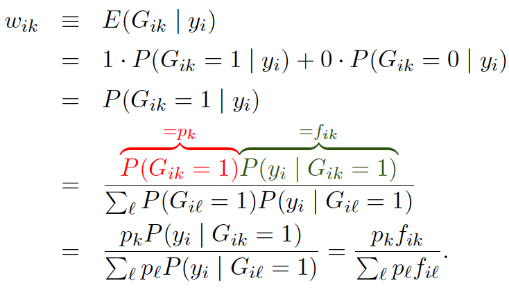
Idea: Give the likelihood some more ‘information.’ Assume that, for an observation $y_i$, we know to which of the $K$ components it belongs; i.e. we assume we know
\[G_{ik} = \begin{cases} 1 & \text{if observation } i \text{ belongs to component } k \\ 0 & \text{otherwise.} \end{cases}\]Then we also know
\[P(G_{ik} = 1 | \theta) = p_k \quad (\text{"prior"})\] \[P(y_i, G_{ik} = 1 | \theta) = P(y_i | G_{ik} = 1, \theta) P(G_{ik} = 1 | \theta) = f_{ik}p_k\]- This gives so-called complete data $(y_i, G_{i1}, \ldots, G_{iK})$, $i = 1, \ldots, n$, with
The corresponding likelihood function, called complete likelihood, is
\[L^*(\theta; y_1, \ldots, y_n, G_{11}, \ldots, G_{nk}) = P(y_1, \ldots, y_n, G_{11}, \ldots, G_{nk} | \theta)\] \[= \prod_{i=1}^{n} \prod_{k=1}^{K} (p_k f_{ik})^{G_{ik}}. \tag{1}\]One obtains the complete log-likelihood
\[\ell^* = \log L^* = \sum_{i=1}^{n} \sum_{k=1}^{K} G_{ik} \log p_k + G_{ik} \log f_{ik} \tag{2}\][M Sec 11.4.2.1]
As the $G_{ik}$ are unknown, we replace them by their expectations
This is known as the E-Step. [M Sec 11.4.2.2]
Now we have
\[\ell^* \approx \sum_{i=1}^{n} \sum_{k=1}^{K} w_{ik} \log p_k + w_{ik} \log f_{ik} \quad (3)\]For the M-step, set (in sequence)
\[\frac{\partial \ell^*}{\partial \mu_k} = 0; \quad \frac{\partial \ell^*}{\partial \sigma_k} = 0; \quad \frac{\partial \left( \ell^* - \lambda \left( \sum_{k=1}^{K} p_k - 1 \right) \right)}{\partial p_k} = 0;\]
yielding
\[\hat{\mu}_k = \frac{\sum_{i=1}^n w_{ik} y_i}{\sum_{i=1}^n w_{ik}}; \tag{4}\] \[\hat{\sigma}^2_k = \frac{\sum_{i=1}^n w_{ik} (y_i - \hat{\mu}_k)^2}{\sum_{i=1}^n w_{ik}}; \tag{5}\] \[\hat{p}_k = \frac{\sum_{i=1}^n w_{ik}}{n}. \tag{6}\][M Sec 11.4.2.3]
Example: Solving $\frac{\partial \ell^*}{\partial \mu_k} = 0$
\[\frac{\partial \ell^*}{\partial \mu_k} = \frac{\partial}{\partial \mu_k} \sum_{i=1}^{n} \sum_{\ell=1}^{K} w_{i\ell} \log p_\ell + w_{il} \log fil\] \[= \frac{\partial}{\partial \mu_k} \sum_{i=1}^{n} \sum_{\ell=1}^{K} w_{i\ell} \log p_\ell + w_{il} \log fil\] \[= - \sum_{i=1}^{n} w_{ik} \left( \frac{(y_i - \mu_\ell)^2}{2\sigma_\ell^2} \right)\]So
\[\iff \sum_{i=1}^{n} w_{ik} y_i = \hat{\mu}_k \sum_{i=1}^{n} w_{ik}\] \[\iff \sum_{i=1}^{n} w_{ik} (y_i - \hat{\mu}_k) = 0\] \[\iff \hat{\mu}_k = \frac{\sum_{i=1}^{n} w_{ik} y_i}{\sum_{i=1}^{n} w_{ik}}.\]==tobe xiugai==
EM Output
Cycling between the E-step and M-step until convergence, leads to two sorts of outputs:
Obviously, $\hat{\mu}_k, \hat{p}_k, \hat{\sigma}^2_k, k = 1, \ldots, K.$
But, also a matrix
1
2
of posterior probabilities of component membership.
Useful for clustering and classification!
EM algorithm: Implementation
So, we essentially need to implement only three things:
- The E-Step
- The M-Step
- A wrapper function, which sets some starting values, then cycles between 1. and 2. until some ‘convergence’ is reached, then collects outcomes.
E-Step
1
2
3
4
5
6
7
8
9
10
11
estep <function(dat, p, mu, sigma){
  n <length(dat)
  K <length(mu)
  W <matrix(0, n, K)
  for (i in 1:n){
    W[i,] <p/sigma*exp(-1/(2*sigma^2)*(dat[i]-mu)^2) /
      sum( p/sigma*exp(-1/(2*sigma^2)*(dat[i]-mu)^2)
    }
  }
  return(W)
}
M-Step
1
2
3
4
5
6
7
8
9
10
11
12
13
14
15
16
17
mstep <function(dat, W){
  n <dim(W)[1]
  K <dim(W)[2]

  p <apply(W, 2, sum) / n
  mu <apply(W * dat, 2, sum) / apply(W, 2, sum)

  diff <matrix(0, n, K)
  for (k in 1:K) {
    diff[,k] <- (dat - mu[k])^2
  }

  var <apply(W * diff, 2, sum) / apply(W, 2, sum)
  sigma <sqrt(var)

  return(list("p" = p, "mu" = mu, "sigma" = sigma))
}
The EM algorithm
1
2
3
4
5
6
7
8
9
10
11
12
13
14
15
16
17
18
em <function(dat,K, steps=400){
  p <rep(1/K,K)
  mu <quantile(dat, probs= (1:K)/K-1/(2*K))
  sigma <rep(sd(dat), K)

  s <1
  while (s <= steps){
    W <estep(dat, p, mu, sigma)
    fit <mstep(dat, W)
    p <fit$p
    mu <fit$mu
    sigma <fit$sigma
    s <s + 1
  }

  fit <list("p"=p, "mu"=mu, "sigma"=sigma, "W"=W)
  return(fit)
}
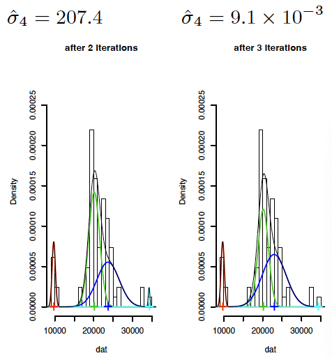
Visualizing the EM algorithm
动态图
Executing the EM algorithm
1
2
3
4
5
6
7
8
9
10
11
12
13
14
15
16
17
18
19
20
21
22
23
24
25
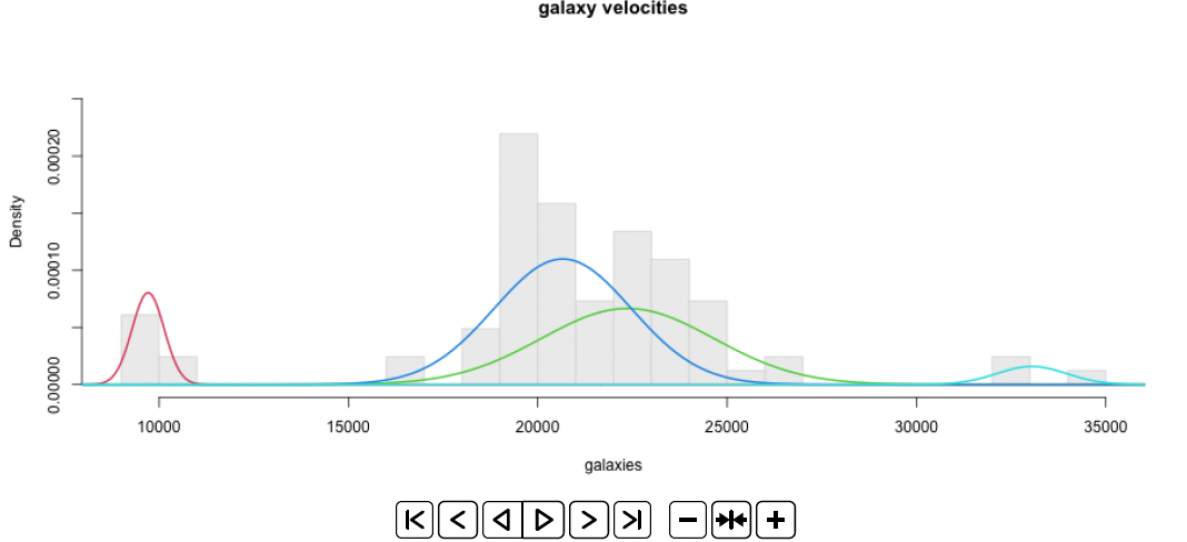
fit.em1 <em(galaxies, K=4)
fit.em1$mu
## [1] 9710.143 23185.905 19964.860 33044.335
fit.em1$sigma
## [1] 422.5107 1633.3574 1385.2894 921.7177
fit.em1$p
## [1] 0.08536585 0.39123845 0.48681039 0.03658531
fit.em2 <em(energy01, K=2)
fit.em2$mu
## [1] 6.321075 8.080906
fit.em2$sigma
## [1] 0.5259982 0.6735426
fit.em2$p
## [1] 0.4769274 0.5230726
Visualizing mixture distributions
1
2
3
4
5
6
7
8
9
10
11
12
13
14
15
16
17
18
19
20
21
22
23
24
25
26
27
28
plot.mix<function(dat, p, mu, sigma, breaks=25, dens=TRUE, ngrid=401, ...){
try<hist(dat, breaks=breaks, plot=FALSE)
hist(dat, breaks=breaks, freq=FALSE, ylim=c(0, max(try$density)*1.3),
col="grey93", border="grey85",...)
r <diff(range(dat))
grid<seq(min(dat)-0.15*r, max(dat)+0.15*r, length=ngrid)
K<length(p)
if (length(sigma)==1){
sigma<-rep(sigma, K)
}
grid.mat<matrix(0, ngrid, K)
for (j in 1:K){
grid.mat[,j]<p[j]*dnorm(grid, mu[j], sigma[j])
}
for (j in 1:K){
lines(grid, grid.mat[,j], col=j+1, lwd=2)
}
if (dens){
lines(grid, apply(grid.mat, 1, sum), col=1, lwd=2)
}
invisible()
}
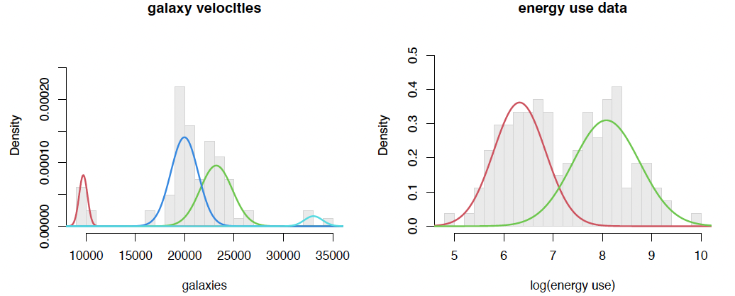
plot.mix(galaxies, fit.em1$p, fit.em1$mu, fit.em1$sigma,
main="galaxy velocities", xlab="galaxies", dens=FALSE)
plot.mix(energy01, fit.em2$p, fit.em2$mu, fit.em2$sigma,
main="energy use data", xlab="log(energy use)", dens=FALSE)
… gives the two plots on Slide 8!
Role of weight matrix: Posterior probabilities of class membership
1
2
3
4
5
6
7
8
9
10
11
12
13
14
15
round(fit.em1$W[1:12,], digits=4)

##      [,1]   [,2]   [,3]   [,4]
## [1,]    1 0.0000 0.0000    0
## [2,]    1 0.0000 0.0000    0
## [3,]    1 0.0000 0.0000    0
## [4,]    1 0.0000 0.0000    0
## [5,]    1 0.0000 0.0000    0
## [6,]    1 0.0000 0.0000    0
## [7,]    1 0.0000 0.0000    0
## [8,]    0 0.0027 0.9973    0
## [9,]    0 0.0029 0.9971    0
## [10,]  0 0.0176 0.9824    0
## [11,]  0 0.0201 0.9799    0
## [12,]  0 0.0211 0.9789    0
1
2
3
4
5
6
7
8
9
10
11
12
round(fit.em2$W[1:9,], digits=4)

##       [,1]    [,2]
## [1,] 0.9672 0.0328
## [2,] 0.8406 0.1594
## [3,] 0.9773 0.0227
## [4,] 0.2409 0.7591
## [5,] 0.9496 0.0504
## [6,] 0.0001 0.9999
## [7,] 0.0016 0.9984
## [8,] 0.3471 0.6529
## [9,] 0.0000 1.0000
… enables using mixtures as a clustering technique, by allocating cases to the component with highest posterior probability (MAP estimation).
Likelihood spikes
Problem: If one data point, say $x_0$, ‘captures’ a mixture component $(\mu_k = x_0$ and $\sigma^2_k \to 0)$, one obtains a solution with infinite likelihood.
Simplistic solution: Set all $\sigma_k \equiv \sigma$. In this case, (5) becomes
Simulation from Gaussian mixtures
This is a two-stage process.
In order to generate a single observation,
- choose a component $k$ from $1, . . . , K$, with probability $p_1, . . . , p_K$;
- sample from the $k$th component, that is from a normal distribution with mean $μk$ and standard deviation $σk$.
Repeat 1. and 2. as many times as required.
1
2
3
4
5
6
7
8
9
10
11
12
13
gauss.mix.sim <function(n, p, mu, sigma){
  x <runif(n)
  sim <rep(0,n)
  cp <cumsum(p)
  for (i in 1:n){
    k <1
    while (x[i] > cp[k]){
      k <k + 1
    }
    sim[i] <rnorm(1, mu[k], sigma[k])
  }
  return(sim)
}
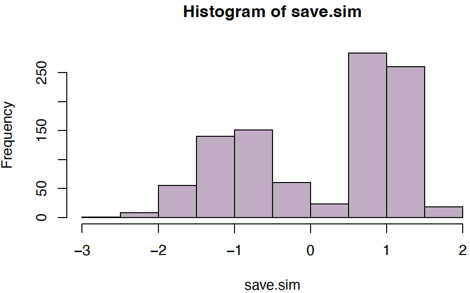
Example: Simulate from mixture with $(\mu_1, \mu_2) = (-1, 1)$, $(\sigma_1, \sigma_2) = (1/2, 1/4)$, and $(p_1, p_2) = (0.4, 0.6)$:
1
2
save.sim <gauss.mix.sim(1000, c(0.4,0.6), c(-1,1), c(1/2,1/4))
hist(save.sim, col="#68246D60")
The number of components
We have so far selected the number $K$ by eye, but this is not ideal; automated criteria are desirable. There is no universally accepted gold standard for this purpose, but the most common methods are as follows.
Use a model selection criterion, such as
\[AIC = -2\log L + 2p\] \[BIC = -2\log L + p\log(n)\]where $L$ is the model likelihood and $p = 3K - 1$ is the total number of model parameters over all components. Minimizing such criteria over $K$ achieves a goodness-of-fit/complexity trade-off. [H Sec 7.6-7.7, M Sec 11.5.1]
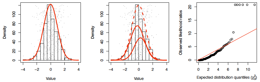
- Use a bootstrap test: For testing $H_0 : K$ versus $H_1 : K + 1$ components,
- fit the model for $K$ and $K + 1$ components to the data at hand, and compute the likelihood ratio (LR) statistic¹;
- generate $B$ samples from the model fitted under $H_0$, and so obtain the null distribution of the LR statistic.
- If the observed LR is among the top 5% of the $B$ bootstrapped LR values, reject $H_0$.
- Use a ‘penalized’ likelihood
¹that is, the difference of the values (-2 \log L) under both models
Multivariate Gaussian mixtures
For multivariate data sets $y_1, \ldots, y_n$, with $y_i \in \mathbb{R}^p$, $i = 1, \ldots, n$, mixture models can in principle be fitted the same way. Now
\[f(y_i | \theta) = \sum_{k=1}^{K} p_k \phi(y_i | \mu_k, \Sigma_k)\]| where $\theta = { p_k, \mu_k, \Sigma_k }_{1 \leq k \leq K}, \mu_k \in \mathbb{R}^p, \Sigma \in \mathbb{R}^{p \times p}$, and the density $f(. | \theta)$ is the density of the MVN as defined in Part I of this module. |
[M Sec 11.2.1]
Model complexity has now increased significantly. We now have:
- $K - 1$ parameters for the mixture probabilities
- $K \times p$ parameters for the component means
- $K \times \frac{p(p + 1)}{2}$ parameters for the component variances
On top of this, we also need to choose $K$!
Model reduction for Multivariate Gaussian mixtures
This large number of parameters is often practically unnecessary, computationally unstable, and leads to overfitting.
Can we reduce the number of parameters somehow?
For the $p_k$ and the $\mu_k$, not much that we can do.
However, the $\Sigma_k$ offer considerable way for simplification, e.g.
(1) all $\Sigma_k$’s are the same; i.e. $\Sigma \equiv \Sigma_k$
(2) all $\Sigma_k$ are diagonal;
(3) all $\Sigma_k$’s are spherical, i.e. diagonal with all values the same;
as well as combinations of (1) with (2) or (3)
Variance parameterizations
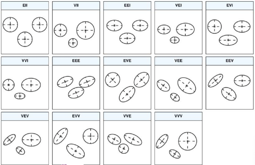
In fact, one can work out that the combination of these three settings enable 14 different types of variance parameterizations, which in R package mclust have been systemized as a three-letter combination:
Does the volume $\det(\Sigma_k)$ of the variance matrices $\Sigma_k$ depend on $k$? Values: E (Equal) or V (Variable)
Does the shape of the variance matrices depend on $k$? Values: I: Spherical; E: (not spherical and equal); V (not spherical and variable).
Does the orientation depend on $k$? Values: I: Diagonal; E (not diagonal but equal); V (not diagonal but variable).
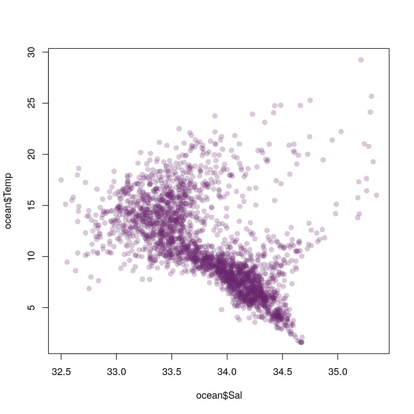
Example: Ocean data
Pacific water temperature data. Interested in joint distribution of water temperature and salinity
1
2
3
4
5
6
ocean <- read.table(
  "http://www.maths.dur.ac.uk/~dma0je/Data/ocean.dat",
  header=TRUE, sep=","
)

plot(ocean$Sal, ocean$Temp, col="#68246d40", pch=16)
Density estimation with mclust
The mclust function will optimize BIC over all values of K and all possible variance parametrizations; and automatically fit the relevant mixture model:
1
2
3
4
require(mclust)
set.seed(105)
ocean.fit <Mclust(cbind(ocean$Sal, ocean$Temp))
plot(ocean.fit, what="BIC")
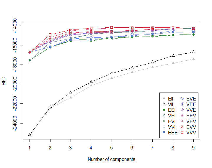
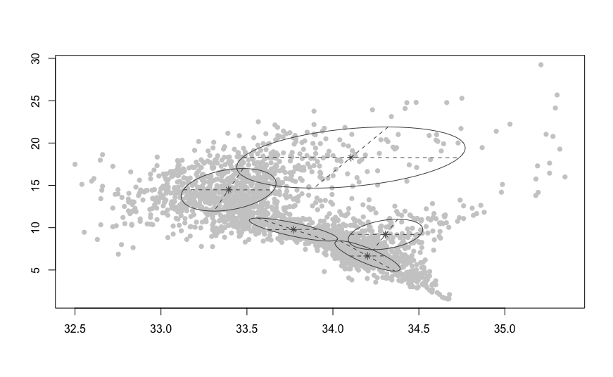
Note that, in this case, the BIC-optimal² solution is VVV (ellipsoidal, varying volume, shape, and orientation) model with $K = 5$ components; i.e. all variance matrices $\Sigma_k, k = 1, \ldots, 5$ are different and fully parametrized.
1
2
3
plot(ocean.fit, what="classification",
col="grey80", symbols=rep(16, 5))
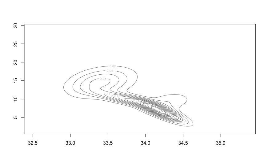
plot(ocean.fit, what="density")
² Note that the values of BIC reported by mclust are actually “minus BIC” according to our earlier definition.
Practical 2
In the second lab session (fetch Practical 2 on Jupyter), we will:
- focus on mixture models;
- compare results to the built-in function normalmixEM in R package mixtools;
- implement the bootstrap methodology for testing the number of components;
- enhance our function em slightly so that it also calculates and displays the model likelihood;
Revisiting estimation of K
Estimating the number of components K is generally of interest. Our ‘bootstrap’ approach (from earlier slides) is useful, but has drawbacks:
- Our true distribution might not be mixture normal at all
- We can’t be sure we’ve found maximum likelihood estimates
- Likelihood spikes: maximum likelihood may be infinite
- The null distribution we derive depends on the data we are testing
Likelihood ratios and Wilks’ theorem (not examinable)
An extremely useful general method for seeing whether we are justified in making a model more complicated is Wilks’ theorem.
Roughly:
Suppose we have two options to model a dataset $X = (x_1, x_2, \ldots, x_n)$: using a ‘more complicated model (MCM)’ $f(x; \theta, \phi)$ or a ‘less complicated model (LCM)’ $f(x; \theta, \phi = \phi_0)$, with $ \phi = p$. - Let $L_1(x) = \max_{\theta,\phi} \prod_i f(x; \theta, \phi)$ be the maximum likelihood of $X$ under MCM, and $L_0(x) = \max_{\theta} \prod_i f(x; \theta, \phi = \phi_0)$ the maximum likelihood under LCM.
Then if $X$ follows the LCM, as $n \to \infty$ we have
\[LR = -2\log\left(\frac{L_1(X)}{L_2(X)}\right) \xrightarrow{d} \chi^2_p\]Example: does sex has affect HDL cholesterol (ind. of age)?
3Proof (heavy going): <www.math.umd.edu/~slud/s701.S14/WilksThm.pdf>
Likelihood ratios and Wilks’ theorem
We have data and models
\[D = \begin{pmatrix} \text{Chol.} & \text{Age} & \text{Sex} \\ 3.1 & 52 & F \\ 4.2 & 43 & M \\ 2.5 & 31 & F \\ \vdots & \vdots & \vdots \\ \end{pmatrix}\]LCM: $f(\text{Chol.} \mid \beta_1, \sigma) = N(\beta_1 \cdot \text{Age}, \sigma^2)$
MCM: $f(\text{Chol.} \mid \beta_1, \sigma) = N(\beta_1 \cdot \text{Age} + \beta_2 \cdot \text{Sex}, \sigma^2)$
Now $\theta = {\beta_1, \sigma}; \phi = {\beta_2}; \phi_0 = 0.$
Suppose we find $LR = 6$: now we can roughly say the probability of seeing $LR > 6$, if the data follow the LCM, is $P(\chi^2_1 > 6) = 0.008$
Wilks theorem for Gaussian mixtures?
What if we try the same for Gaussian mixtures?
LCM: $f(x; \theta) = \phi(x; \mu_1, \sigma_1);$
MCM: $f(x; \theta, \phi) = p_1 \phi(x; \mu_1, \sigma_1) + (1 - p_1) \phi(x; \mu_2, \sigma_2)$
so $\theta = (\mu_1, \sigma_1); \phi = (p_1, \mu_2, \sigma_2)$
Identifiability
Unfortunately, Wilks’ theorem doesn’t hold here!
One important condition for Wilks’ theorem to hold is identifiability: if we take enough samples we can eventually identify $\theta, \phi$ arbitrarily well.
But if the data follow the LCM, we can never identify $p_1$: these three models describe the same distribution (which is just $\phi(x; 0, 1)$):
$\frac{1}{2} \phi(x; 0, 1) + \frac{1}{2} \phi(x; 0, 1)$ ((\theta = (1, 0); \phi = (\frac{1}{2}, 1, 0)))
$\frac{1}{10} \phi(x; 0, 1) + \frac{9}{10} \phi(x; 0, 1)$ ((\theta = (1, 0); \phi = (\frac{1}{10}, 1, 0)))
$1 \times \phi(x; 0, 1) + 0 \times \phi(x; -10, \frac{1}{5})$ ((\theta = (1, 0); \phi = (\frac{1}{2}, -10, \frac{1}{5})))
等待修改
penalized likelihood for Gaussian mixtures
It turns out we can make Gaussian mixture models identifiable and sort out likelihood spikes, in one fell swoop:
\[\ell^p(\theta; y_1, \ldots, y_n) = \sum_{i=1}^n \log\left(\sum_{k=1}^K p_k f_{ik}\right) + C \log\left(\prod_{k=1}^K p_k\right)\]The only change to the E-M algorithm is:
\[w_{ik} = \frac{p_k f_{ik} + C}{\sum_{\ell} p_\ell f_{i\ell} + KC}\]This makes sense, because we are essentially adding $C$ ‘phantom’ points to each cluster. Wilks’ theorem can now be used.
Chen, Hanfeng, Jiahua Chen, and John D. Kalbfleisch. “A modified likelihood ratio test for homogeneity in finite mixture models.” Journal of the Royal Statistical Society: Series B (Statistical Methodology) 63.1 (2001): 19-29.
Kernel Density Estimation (examinable again)
The methods discussed so far are referred to as parametric, since their distributional shape is specified up to some parameters (which need to be estimated).
There is the risk of mis-specifying the parametric shape (which was, in our case, Gaussian) or the number of components.
We want methods for density estimation which do not make such assumptions. Such methods are called nonparametric.
Kernel Density Estimation
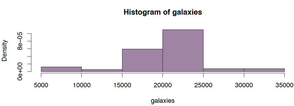
Return to the galaxy velocities example.
Note that a histogram is a simple nonparametric density estimator [C Sec 2.1].
Produce histograms using the default settings in R:
1
2
data(galaxies, package="MASS")
hist(galaxies, freq=FALSE, col="#68246d90")
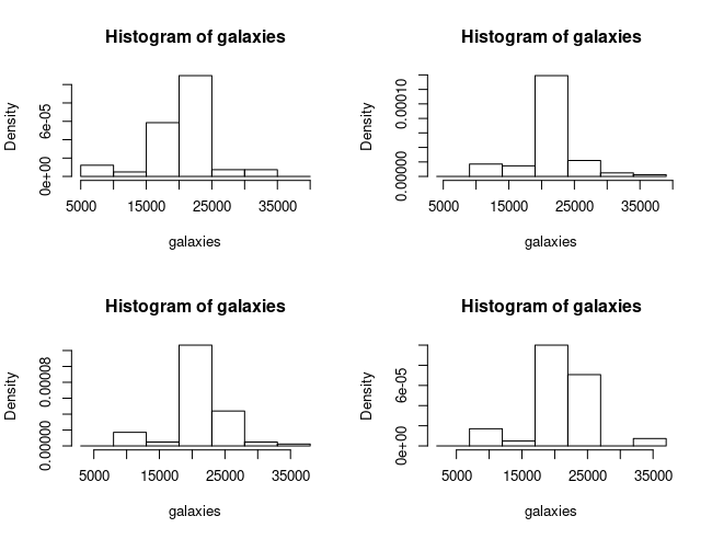
Even with the same number of bins (but a different anchor point for the first bin), histogram shapes for the same data can differ drastically…
1
2
3
4
5
6
7
8
9
par(mfrow=c(2,2))
hist(galaxies, freq=FALSE,
     breaks=seq(5000, 40000, by=5000))
hist(galaxies, freq=FALSE,
     breaks=seq(4000, 39000, by=5000))
hist(galaxies, freq=FALSE,
     breaks=seq(3000, 38000, by=5000))
hist(galaxies, freq=FALSE,
     breaks=seq(2000, 37000, by=5000))
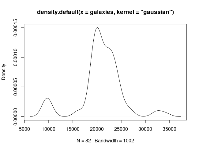
Histograms are ‘not smooth’. Nature usually is…
We would like something like:
1
plot(density(galaxies, kernel="gaussian"))
This can be achieved through kernel density estimation.
Consider the problem of naively estimating a density $f(\cdot)$ from data $x_1, \ldots, x_n$:
\[\hat{f}(x) = \frac{1}{2h} \left\{ \#\{x_i : x_i \in (x - h, x + h)\} \right\} = \frac{1}{nh} \sum_{i=1}^n K\left( \frac{x - x_i}{h} \right)\]using the uniform kernel: $K(u) = \frac{1}{2}$ if $-1 < u \leq 1$ and $0$ otherwise.
We apply this estimator on the galaxy data:
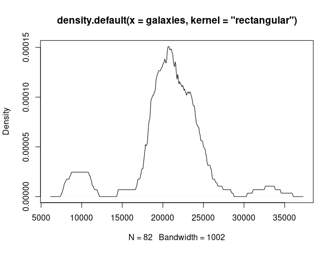
1
plot(density(galaxies, kernel="rectangular"))
This is quite wiggly! Problem: The kernel that we used is “unsmooth”. Consequence: We need better (smoother) kernels!
[M Sec 14.7.2]
For instance, we may use a Gaussian density for $K$.
The resulting kernel density estimator
\[\hat{f}(x) = \frac{1}{nh} \sum_{i=1}^{n} K \left( \frac{x - x_i}{h} \right)\]estimates the density by redistributing the point mass $\frac{1}{n}$ smoothly to its vicinity.
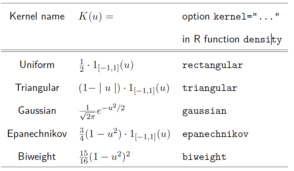
Generally, a kernel function $K$ is symmetric, bounded, and non-negative, with
\[\int K(u) \, du = 1. \text{ (Exceptions exist!)}\]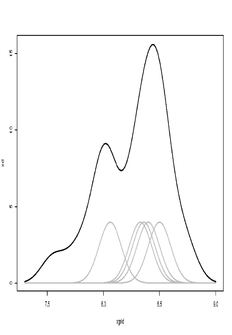
Commonly used kernel functions
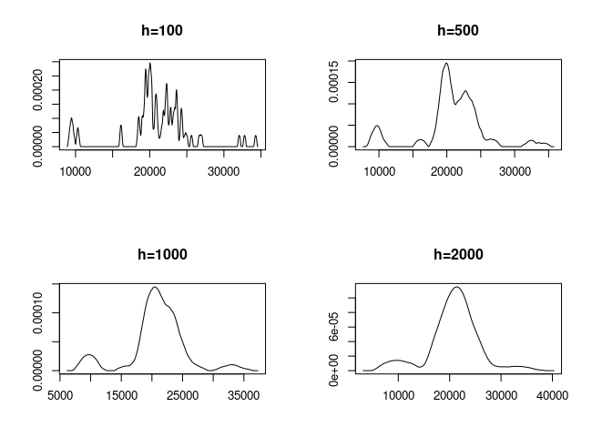
Effect of bandwidth
For different kernels $K$, the results are more or less similar as long as the kernel is ‘smooth’. Far more important than the choice of the kernel is the choice of the bandwidth $h$.
1
2
3
4
5
6
7
8
9
par(mfrow=c(2,2))
plot(density(galaxies, kernel="epanechnikov", adjust=0.1),
     xlab="", ylab="", main="h=100")
plot(density(galaxies, kernel="epanechnikov", adjust=0.5),
     xlab="", ylab="", main="h=500")
plot(density(galaxies, kernel="epanechnikov"),
     xlab="", ylab="", main="h=1000")
plot(density(galaxies, kernel="epanechnikov", adjust=2),
     xlab="", ylab="", main="h=2000")
h too small
undersmoothing
Bandwidth selection
Silverman’s ‘normal reference’ rule of thumb:
\[h_{\text{opt}} = 0.9A n^{-1/5}\]with $A = \min(\text{st.dev.}, IQR/1.34)$.
Based on minimizing the asymptotic mean integrated squared error.
Many alternative bandwidth selection methods exist, but this one is the simplest, computationally fastest, and works generally well.
Bivariate density estimation
For bivariate data $x_1, \ldots, x_n \in \mathbb{R}^2$ we need a bivariate kernel $K : \mathbb{R}^2 \to \mathbb{R}$, which can either be realized through a product kernel (generated from a univariate kernel $K$):
\[K^P(u_1, u_2) = K(u_1)K(u_2)\]or through a radially symmetric kernel
\[K^S(u_1, u_2) = \text{const} \cdot K\left(\sqrt{u_1^2 + u_2^2}\right)\]If $K$ is a Gaussian kernel, then $K^P$ and $K^S$ are equivalent, and one gets
\[K(u_1, u_2) = \frac{1}{2\pi} \exp\left(-\frac{1}{2}(u_1^2 + u_2^2)\right)\]
Bivariate Gaussian kernel:
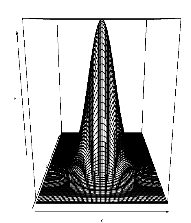
We need then two bandwidths $h_1$ and $h_2$ controlling the smoothness of the fit in direction of the corresponding axes. The estimate of the “true” density $f(x_1,x_2)$ is given by
\[\hat{f}(x_1,x_2) = \frac{1}{nh_1 h_2} \sum_{i=1}^{n} K \left( \frac{x_1 - x_{i1}}{h_1}, \frac{x_2 - x_{i2}}{h_2} \right)\]Sometimes one will set $h_1 = h_2 = h$. This is only sensible if $X_1$ and $X_2$ are measured in the same units, or are appropriately standardized. We refer to this as the isotropic bandwidth choice.
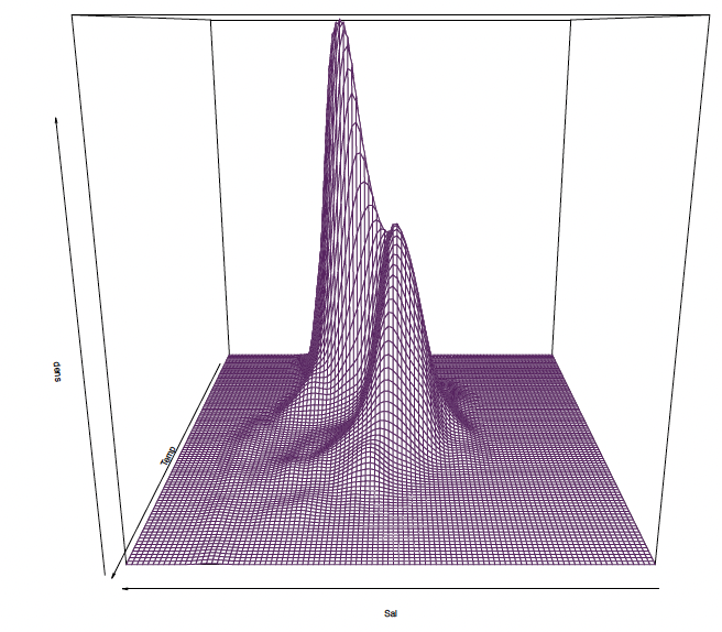
Bivariate density estimation
Return to ocean data
1
2
3
4
5
6
7
require(MASS)
ocean.kde <kde2d(ocean$Sal, ocean$Temp, n=100, lims=c(31,36,0,30))
dim(ocean.kde$z)

## [1] 100 100

persp(ocean.kde$z, theta=180, border="#68246d", xlab="Sal", ylab="Temp", zlab="dens")
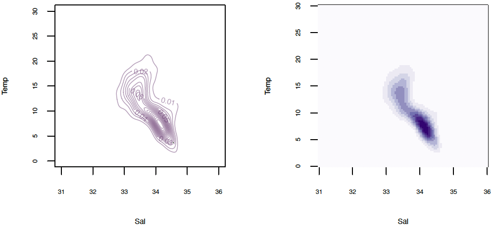
Alternatively, the estimated density can also be visualized through contour or image plots:
1
2
3
4
5
6
par(mfrow=c(1,2), cex.lab=0.6, cex.axis=0.5)
library(RColorBrewer)
contour(ocean.kde$x, ocean.kde$y, ocean.kde$z,
        xlab="Sal", ylab="Temp", nlevels=20, col="#68246D70")
image(ocean.kde$x, ocean.kde$y, ocean.kde$z,
      xlab="Sal", ylab="Temp", col=brewer.pal(9, "Purples"))
Multivariate density estimation
The concept generalizes immediately to data of any dimension [C Sec 2.2]. Let $x_1, \ldots, x_n \in \mathbb{R}^p$. The $p$-variate kernel density estimator of $f$ is given by
\[\hat{f}(x) = \frac{1}{n | H |^{1/2}} \sum_{i=1}^{n} K(H^{-1/2}(x - x_i))\]where
\[K(u) = (2\pi)^{-p/2} \exp\left(-\frac{1}{2} u^T u\right)\]and
\[H = \text{diag}(h_1^2, \ldots, h_p^2)\]is a bandwidth matrix. This amounts to summing the multivariate normal densities, $N(x_i, H)$.
Bandwidth selection for multivariate density estimation
By extending the “normal reference” bandwidth selector to dimensions $p > 1$, an optimal bandwidth matrix is derived to be
\[H = \left( \frac{4}{p+2} \right)^{\frac{2}{p+4}} n^{-\frac{2}{p+4}} \hat{\Sigma}\]where $\hat{\Sigma}$ is the estimated variance matrix. Assuming diagonal form, $H = \text{diag}(h_1^2, \ldots, h_p^2)$, this gives
\[h_j = \left( \frac{4}{p+2} \right)^{\frac{1}{p+4}} n^{-\frac{1}{p+4}} \hat{\sigma}_j\]for the component bandwidths (with $\hat{\sigma}_j$ being the standard deviation of the $j$th variable). Now, noting that the leading term is $\approx 1$, one has the surprisingly simple formula (Scott’s rule in $\mathbb{R}^p$, [C Sec 3.1])
\[h_j = \hat{\sigma}_j n^{-\frac{1}{p+4}}.\]