UL3

UL Part 3: Clustering

Overview over Part 3

We will…

• explain how mixture models can be used for clustering via the maximum a posteriori rule;
• explain how kernel density estimation can be used for clustering, via
  • high density regions;
  • density modes and the mean shift algorithm;
• discuss how to assess the goodness-of-fit of clustering techniques (being related to the choice of the number of clusters); particularly the elbow method, the gap statistic, silhouettes, and the Rand index.

Clustering

Clustering is the process of partitioning a data set $\mathcal{Y} = (y_1, \ldots, y_n)^T$, with $y_i \in \mathbb{R}^d$, into disjoint subsets $C_k, k = 1, \ldots, K$ (called clusters), so that those elements within each cluster are more similar to each other than elements in different clusters [J Sec 10.3].

Most clustering techniques accomplish this aim in two steps:

• Find the cluster centers;
• Assign all observations to one of the centers.

We have already seen two clustering techniques in Part I, which achieve this: $k$-means and $k$-medoids.

Recall: $k$-means for Wally’s data

wally.kmean <kmeans(wally.pts[,c("X","Y")], centers=3)
wally.kmean$centers

##       X          Y
## 1  6.443841  4.804348
## 2 10.978261  4.237319
## 3  2.497475  2.525568

head(wally.kmean$cluster)

## [1] 3 1 1 1 1 1

plot(wally.pts$X, wally.pts$Y, 
     col=wally.kmean$cluster, pch=16)
points(wally.kmean$centers,
       col=c(1,2,3), pch=10, cex=2)

library(clue)
wally.kmed <kmedoids(dist(wally.pts[,c("X","Y")]), k=3)
wally.kmed$medoid_ids
## [1] 23 50 53
head(wally.kmed$cluster)
## [1] 1 2 2 2 2 2

plot(wally.pts$X, wally.pts$Y,
     col=wally.kmed$cluster, pch=16)
points(wally.pts$X[wally.kmed$medoid_ids],
       wally.pts$Y[wally.kmed$medoid_ids],
       col=c(1,2,3), pch=9, cex=2)

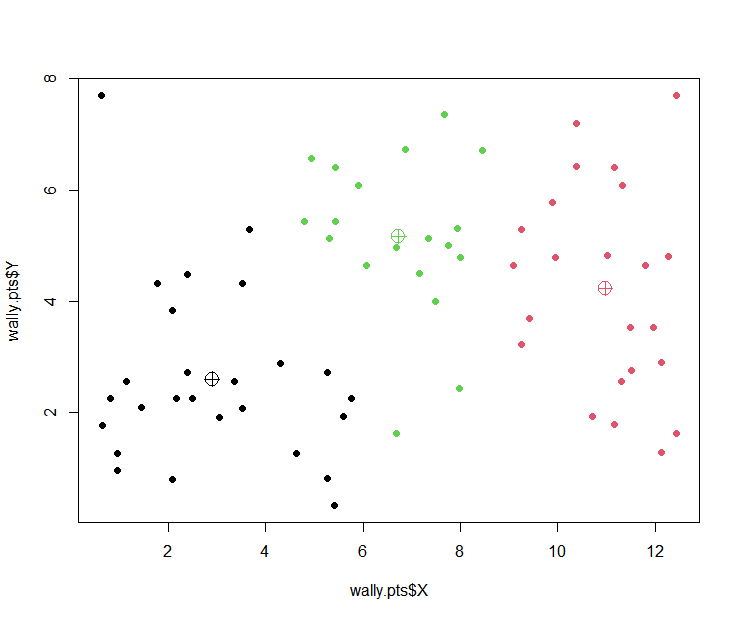
Mixtures and Clustering

It is clear that the mixture centers are natural candidates for cluster centers:

require(mixtools)
wally.mix <mvnormalmixEM(wally.pts[,c("X","Y")], k=3)
wally.mix$mu

[[1]]
[1] 3.172080 2.599816

[[2]]
[1] 6.507791 5.318982

[[3]]
[1] 10.612284 4.448306

(The R function mvnormalmixEM is a simple multivariate version of our implementation em, in contrast to the high-level function mclust).

How does the cluster assignment work?

Recall we do have the posterior probabilities of class membership:

head(round(wally.mix$posterior, digits=4))\

	comp.1	comp.2	comp.3
[1,]	0.9953	0.0047	0.0000
[2,]	0.0295	0.9695	0.0010
[3,]	0.0173	0.9804	0.0023
[4,]	0.0116	0.9840	0.0044
[5,]	0.0477	0.9542	0.0010
[6,]	0.1364	0.8633	0.0003

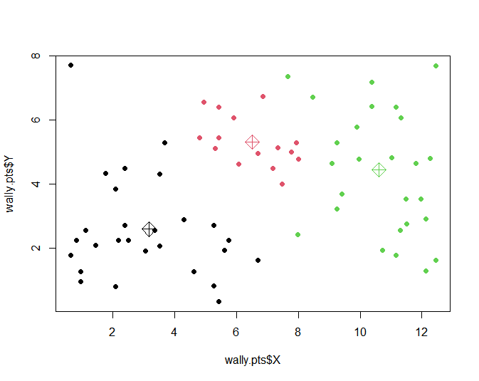
MAP clustering for mixtures

By the maximum a posteriori (MAP) rule, we allocate each observation to the mixture center to which it belongs with maximum probability [H Sec 14.3.7]:

wally.cluster <apply(wally.mix$posterior, 1, which.max)
wally.cluster

[1]  1 2 2 2 2 2 2 1 2 1 1 1 1 1 1 1 1 1 1 1 1 1 1 1 1 1 1 1
[29] 1 1 1 1 1 3 2 3 3 3 3 3 3 3 3 3 3 3 2 2 2 2 2 2 2 2 3 3
[57] 3 3 3 3 1 3 3 3 3 3 3 3

plot(wally.pts$X, wally.pts$Y, col=wally.cluster, pch=16)
mu <matrix(unlist(wally.mix$mu), ncol=2, byrow=TRUE)
points(mu, col=c(1,2,3), pch=9, cex=2)

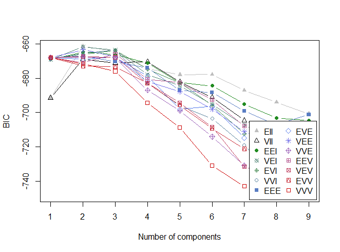
Clustering via mclust

Just as for the density estimation problem, mclust can be used for automatic determination of model complexity via BIC:

wally.mixx <Mclust(wally.pts[,c("X", "Y")])
plot(wally.mixx)

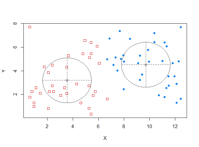
In this case, mclust chooses the most simple 2-component model (EII):

Resulting clustering according to MAP rule:

Connection between EM algorithm and k-means

The similar results using EM and k-means are not coincidental. The EM algorithm and k-means are very closely connected. Consider the EM algorithm, set all variances to $\sigma^2_k = 1$ and $p_k = \frac{1}{K}$ for all $k = 1, \ldots, K$. Instead of computing the individual cluster membership probabilities, we assign each data point to the most likely cluster

\[{argmax} _k P(G_{ik} = 1 | y_i) = {argmin} _k \| y_i - \mu_k \|^2.\]

The weights $w_{ik}$ are now either 1 if $i$ is in cluster $k$ and 0 otherwise, equation (4) from Part 2 Slide 15 reduces to the cluster mean

\[\mu_k = \frac{1}{|C_k|} \sum_{i \in C_k} y_i.\]

[M Section 11.4.2.5]

Clustering through density estimation

Recall: Bivariate kernel density estimate (using for instance a bivariate Gaussian kernel, $K(x_1,x_2) = \frac{1}{2\pi} \exp\left{-\frac{1}{2}(x_1^2 + x_2^2)\right}$,

\[\hat{f}(x_1,x_2) = \frac{1}{nh_1h_2} \sum_{i=1}^{n} K\left( \frac{x_1 - x_{i1}}{h_1}, \frac{x_2 - x_{i2}}{h_2} \right)\]

For instance, to use $h_1 = h_2 = 1$, we define a bandwidth matrix $[C \text{ Sec } 2.2]$

\[H = \begin{pmatrix} h_1^2 & 0 \\ 0 & h_2^2 \end{pmatrix} = \begin{pmatrix} 1^2 & 0 \\ 0 & 1^2 \end{pmatrix} = \begin{pmatrix} 1 & 0 \\ 0 & 1 \end{pmatrix}\]

H = diag(1,2)  
H  
## [,1] [,2]  
## [1,] 1 0  
## [2,] 0 1  

… and then execute:

require(ks)  
wally <wally.pts[,c("X", "Y")]  
wally.ks <kde(wally, H=H, gridsize=200)  
plot(wally.ks)  
points(wally.pts$X, wally.pts$Y, col=2)  

or, as a perspective plot:

plot(wally.ks,
     display="persp",
     theta=30)

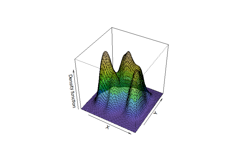The images convey a notion that “density bumps correspond to clusters”.

A traditional technique to quantify this idea are level sets, that is regions of the data domain which exceed a density threshold, say $c$:

\[\mathcal{L}(c) = \{x | \hat{f}(x) > c\}.\]

For $c$ it is common to use a value such $c_\alpha$ such that

\[\int_{\mathcal{L}(c_\alpha)} \hat{f}(x) \, dx = 1 - \alpha.\]

[C Sec 6.1]

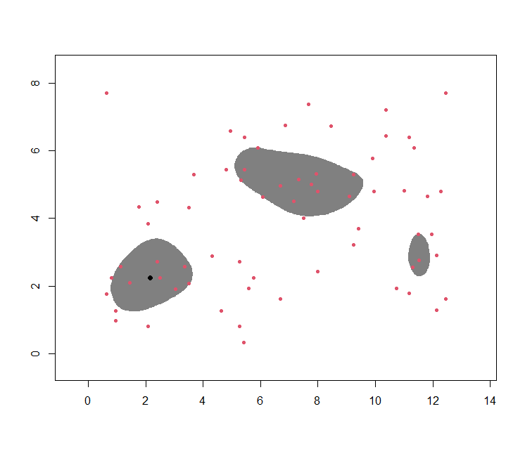
High density region

This latter concept is also referred to as a high density region (HDR): For instance, the following gives a 70% HDR:

require(hdrcde)
wally.hdr <hdr.2d(wally.pts$X, wally.pts$Y,
    prob=0.7, kde.package="ks", h=c(1,1))
wally.hdr$alpha  # cut-off constant c
## 
## 70%
## 0.01447569

plot(wally.hdr, show.points=TRUE, pointcol=2)

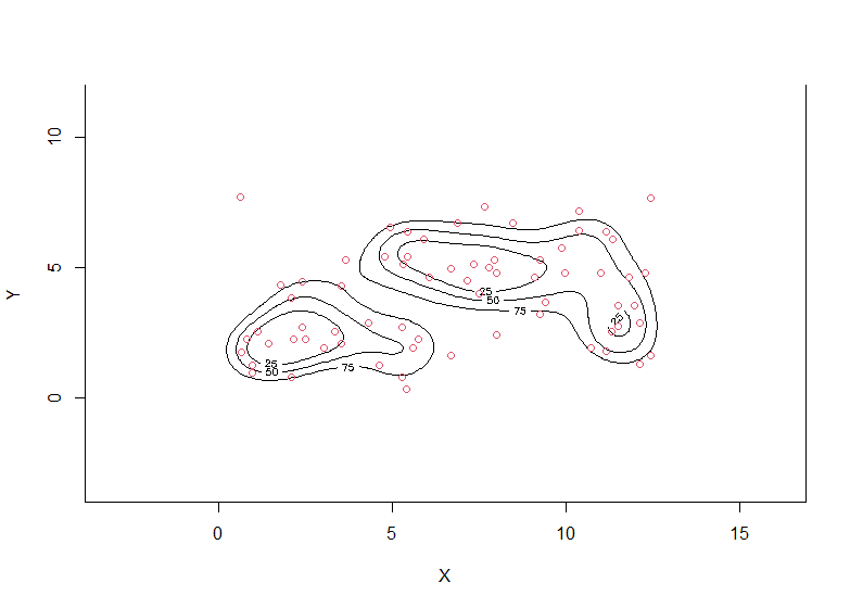
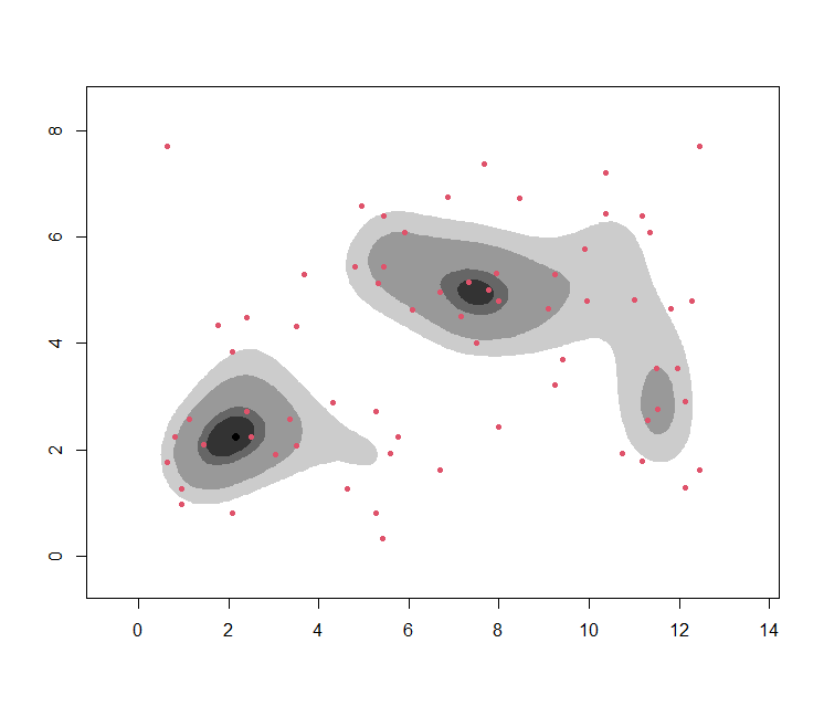
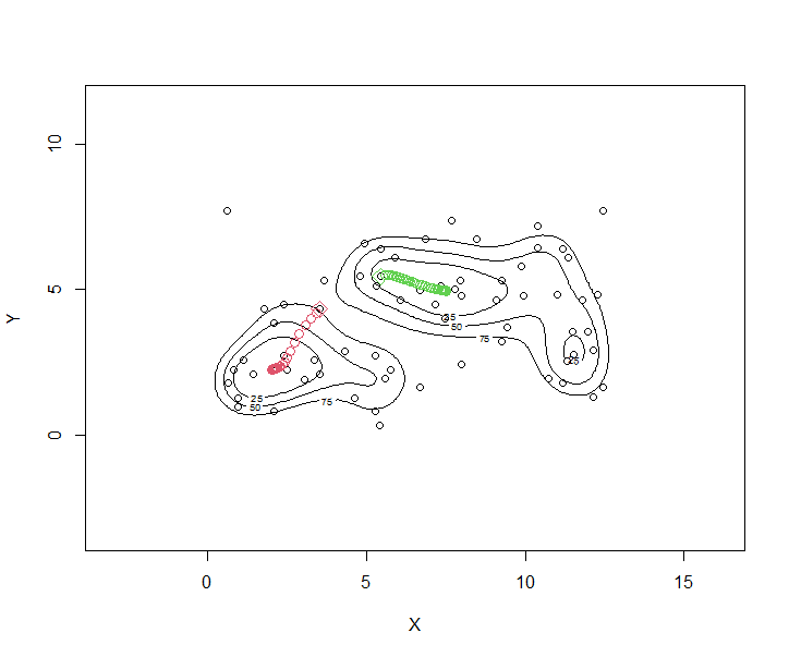
One can also do this for several values of $\alpha$ at once, then coinciding with the concept of a contour plot:

wally.hdr <hdr.2d(wally.pts$X, wally.pts$Y,
                    kde.package="ks", h=c(1,1),
                    prob=c(0.5,0.7,0.9,0.95))
plot(wally.hdr, show.points=TRUE, pointcol=2)

Limitations of HDRs

HDRs (or level sets) themselves have a few limitations:

• The choice of the threshold $c$ is somewhat arbitrary.

• The approach fails to qualify as a ‘clustering’ method in the sense of our definition, since not all data can be associated to a HDR (or the HDRs start overlapping and hence the allocation becomes ambiguous)

Hence, alternative ways of density-based clustering are desirable!

Overall mode

Observe the black dot in the previous images. This is the overall mode, i.e. the maximum of $\hat{f}$:

\[\text{Mode} = \arg \max_x \hat{f}(x).\]

hdrcde computes this point simply through a grid search (which evaluates the density over a mesh of grid points, and then identifies that one yielding the maximum density).

wally.hdr$mode
[1] 2.166667 2.250000

#$

Local modes as cluster centers?

Conceptually, it appears sensible to identify cluster centers with all local modes.

However, a grid search is not very effective for this, since it is

• computationally very demanding (and may become actually infeasible if, say, $p \geq 3$)
• is not-so-easy to implement if one is interested in all local modes, not just the global one.

(Indeed, hdrcde cannot do this.)

Estimation of density modes

Systematic approach: Modes can be estimated as extremal points of the density; i.e. points with

\[\nabla \hat{f}(x) = 0.\]

It turns out that, in order to execute this derivation efficiently, it is beneficial to rewrite the kernel $K(x)$ as $k(|x|^2)$, with Euclidean norm $|x|^2 = x_1^2 + \cdots + x_p^2$, where the profile $k: \mathbb{R} \to \mathbb{R}$ is a non-negative function such that

\[\int_{\mathbb{R}^d} k(\|x\|^2)dx = 1.\]

For instance, for the multivariate Gaussian kernel, one has

\[k(u) = (2\pi)^{-p/2} e^{-u/2}\]

and so

\[K(x) = (2\pi)^{-p/2} e^{-\|x\|^2/2}.\]

With this formulation, one can write the density estimate as

\[\hat{f}(x) = \frac{1}{n|H|^{1/2}} \sum_{i=1}^{n} K(H^{-1/2}(x_i - x))\] \[= \frac{1}{n|H|^{1/2}} \sum_{i=1}^{n} k(\|H^{-1/2}(x_i - x)\|^2)\]

and some algebra shows that its gradient is given by

\[\nabla \hat{f}(x) = -\frac{2}{n|H|^{1/2}} H^{-1} \sum_{i=1}^{n} k'(\|H^{-1/2}(x_i - x)\|^2)(x_i - x)\]

Equating $\nabla \hat{f}(x) = 0$, one obtains the iterative equation

\[x = \frac{\sum_{i=1}^{n} k' \left( \| H^{-1/2}(x_i - x) \|^2 \right) x_i}{\sum_{i=1}^{n} k' \left( \| H^{-1/2}(x_i - x) \|^2 \right)}\]

For the special case of a Gaussian profile, one has $k’(u) = -\frac{1}{2} k(u)$, and so

\[x = \frac{\sum_{i=1}^{n} k \left( \| H^{-1/2}(x_i - x) \|^2 \right) x_i}{\sum_{i=1}^{n} k \left( \| H^{-1/2}(x_i - x) \|^2 \right)},\]

equivalently

\[x = \frac{\sum_{i=1}^{n} K(H^{-1/2}(x_i - x))x_i}{\sum_{i=1}^{n} K(H^{-1/2}(x_i - x))}.\]

A mode of $\hat{f}$ corresponds to a point $x$ which solves (2).

This equation does not have an analytical solution. However, one can arrive at a solution by executing the right side of (2) iteratively, i.e. beginning from some starting point $x^{(\ell)}$, one iterates

\[x^{(\ell)} = \frac{\sum_{i=1}^n K(H^{-1/2}(x_i - x^{(\ell-1)}))x_i}{\sum_{i=1}^n K(H^{-1/2}(x_i - x^{(\ell-1)}))}\]

One can show that

• the mean shift $x^{(\ell+1)} - x^{(\ell)}$ is proportional to $\frac{\nabla \hat{f}(x^{(\ell)})}{\hat{f}(x^{(\ell)})}$;
• the sequence of $x^{(\ell)}$ always moves in direction of the gradient;
• the sequence of $x^{(\ell)}$ converges to a local mode of $\hat{f}$.

Sequence of $x^{(\ell)}$ for two arbitrarily selected starting points; using fixed $(h_1,h_2) = c(1,1)$.

(code on next page)

require(LPCM)
x1 <c(wally.pts$X[10], wally.pts$Y[10])
ms.x1 <ms.rep(wally.pts[,c("X", "Y")], x=x1, h=1)
x2 <c(wally.pts$X[5], wally.pts$Y[5])
ms.x2 <ms.rep(wally.pts[,c("X", "Y")], x=x2, h=1)

plot(wally.ks)
points(wally.pts$X, wally.pts$Y)
points(wally.pts$X, wally.pts$Y)
points(x1[1], x1[2], col=2, pch=5, cex=1.5)
points(x2[1], x2[2], col=3, pch=5, cex=1.5)
points(ms.x1$Meanshift.points, col=2, cex=1.2)
points(ms.x2$Meanshift.points, col=3, cex=1.2)

Mean shift clustering

Mean shift trajectories starting from each individual observation.

wally.ms <ms(wally.pts[,c("X", "Y")], scaled=0, h=1)

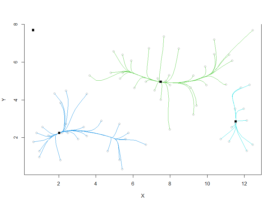We see that once this process is complete, the clustering follows automatically: Each observation is assigned to that cluster to which its trajectory has converged [C Sec 6.2.2]:

wally.ms$cluster.center
     [,1]      [,2]
[1,]  0.6316952 7.695737
[2,]  7.4926538 4.952212
[3,]  2.0306169 2.246337
[4,] 11.5383040 2.852186

wally.ms$cluster.label
 [1] 1 2 2 2 2 2 2 2 3 3 3 3 3 3 3 3 3 3 3 3 3 3 3 3 3 3 3 3 3 3 3 3
[31] 3 3 2 2 2 2 2 2 2 2 2 2 2 2 2 2 2 2 2 2 2 2 2 2 2 2 4 4 2 4 4 2
[61] 3 4 4 4 4 4 4

#$

Goodness-of-fit assessment

We have seen several ways of clustering a given data set. How can we say whether a certain clustering outcome has been more successful than another one?

Specifically, we would be interested in comparing

• clusterings from a particular technique, for different k;
• results from different clustering techniques between each other.

wally <wally.pts[,c("X","Y")]
tot.withinss <rep(0,15)
for (k in 1:15){
  tot.withinss[k] <kmeans(wally,k)$tot.withinss
  #$
}
plot(tot.withinss, type="b", main="Total-within sum of squares")

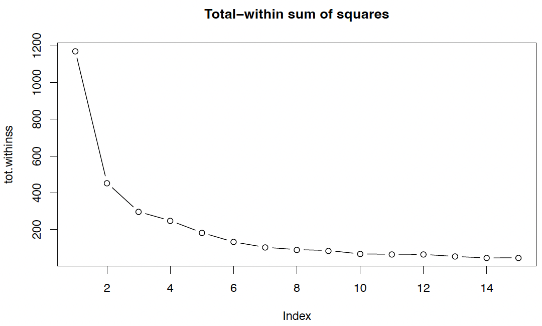
We see that minimizing this criterion is not a constructive strategy.

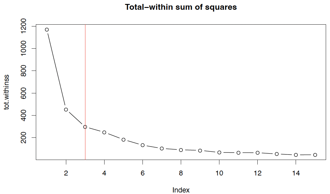
However, a potential solution is given by the elbow method, which defines the ‘elbow’ (bend, kink) from which on an increase of $k$ only gives ‘slow’ improvement.

Here, presumably selects $K = 3$.

plot(tot.withinss, type="b", main="Total-within sum of squares")
abline(v=3, col=2)

Gap statistics

Clearly, the elbow method is somewhat ambiguous and subjective!

An approach to formalize this concept through a proper statistical test is the gap statistics, which tests, through the bootstrap, whether the decrease in log-total within-sum of squares is larger than could be expected purely by chance.

require(cluster)
wally.gap<clusGap(wally,FUN=kmeans, K.max = 5, nstart=20, B = 100)
plot(wally.gap)

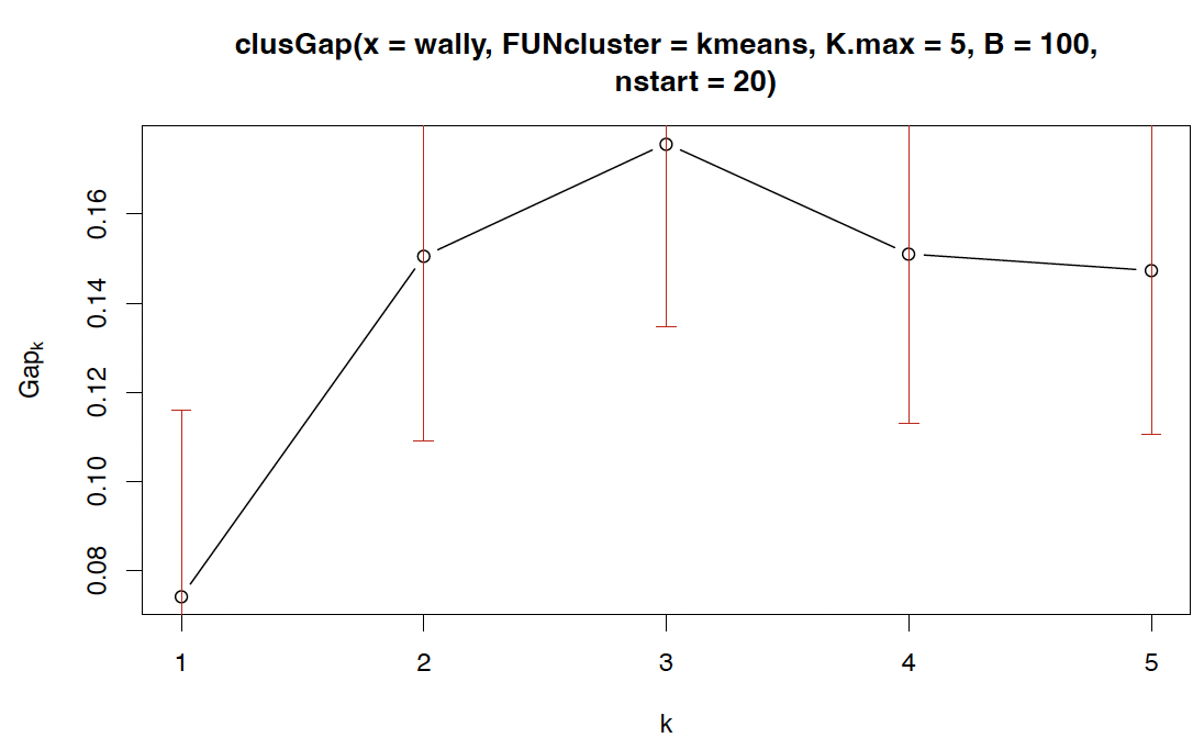
What is displayed here is the ‘gap curve’; i.e. the difference between the expected and the observed log-total within-sum of squares, over different K.

Sensible values of K will produce large values of the gap statistic. Here the maximum is at $K = 3$.

[H Sec 14.3.11] suggest a slightly more complex way of selecting K: Identify the smallest K for which the gap statistic $G_K$ exceeds at least the lower end of error bars (red) at $G_{K+1}$.

Here, this would select $K = 2$ (so the increase from $K = 2$ to $K = 3$ is deemed coincidental).

Silhouettes

A differently motivated measure of goodness-of-fit for a given clustering is obtained by the following strategy:

For each observation $x_i, i = 1, \ldots, n$, identify

• a (dissimilarity) measure $a(x_i)$ of how well $x_i$ fits into its assigned cluster;
• a (dissimilarity) measure $b(x_i)$ of how well $x_i$ would fit into one of the other clusters;
• a measure $s(x_i)$ (‘silhouettes’) of how much smaller $a(x_i)$ is than $b(x_i)$;

Finally, use the average over $s(x_i), \, i = 1, \ldots, n$ to measure the goodness-of-fit (larger is better).

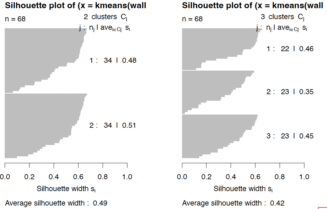
This concept has been applied (mainly for k-means) in the form of silhouette plots.

require(cluster)
par(mfrow=c(1,2))
for (k in 2:3){
  plot(silhouette(kmeans(wally,k)$cluster, dist(wally)))
}

A common choice for these expressions is

\[a(x_i) = \frac{1}{|C(i)| - 1} \sum_{x_j \in C(i), j \neq i} D(x_i, x_j)\] \[b(x_i) = \min_{k: C_k \neq C(i)} \frac{1}{|C_k|} \sum_{x_j \in C_k} D(x_i, x_j)\] \[s(x_i) = \begin{cases} \frac{b(x_i) - a(x_i)}{\max\{a(x_i), b(x_i)\}} & \text{if } |C(i)| > 1 \\ 0 & \text{if } |C(i)| = 1 \end{cases}\]

where $D$ is some dissimilarity such as the Euclidean distance, and $C(i)$ denotes the cluster which includes $x_i$.

The silhouette values $s_i \equiv s(x_i)$ can be interpreted as follows:

• Values of $s_i$ close to 1 mean that case $i$ is well clustered;
• values close to 0 mean that case $i$ could equally well be assigned to another cluster;
• negative values mean that case $i$ would be better assigned to another cluster.

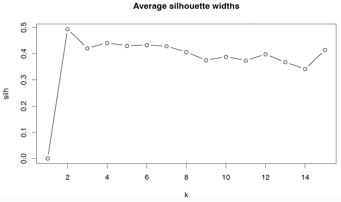
Often, a summary statistic is more useful. Most frequently used is the average silhouette width

\[S = \frac{1}{n} \sum_{i=1}^{n} s_i.\]

silh <rep(0,15)
for (k in 2:15){
  silh[k] <summary(
    silhouette(
      kmeans(wally,k)$cluster,
      dist(wally))
  )$avg.width
}
plot(silh, type="b", main="Average silhouette widths", xlab="k")

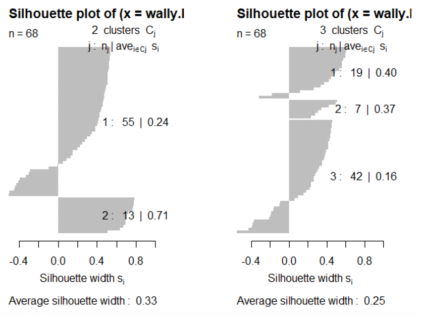
Silhouettes can in principle also be applied to other clustering techniques, although this is not very common:

par(mfrow=c(1,3))
for (k in 2:3){
  wally.kmix <mvnormalmixEM(wally, k=k)
  wally.kcluster <apply(wally.kmix$posterior, 1, which.max)
  plot(silhouette(wally.kcluster, dist(wally)))
}

Other clustering indexes

Similar indexes to the average silhouette width (which define some criterion based on ratios of some sort of intraand between-cluster distances) have been proposed in large number, including

• the Dunn index: the ratio of the smallest distance between observations not in the same cluster to the largest intra-cluster distance (positive index, with infinity corresponding to best clusterings).

• the Davies-Bouldin index: a ratio of a measure of scatter within the cluster and the separation between clusters (positive index, with small values corresponding to good clusterings).

Rand index

The Rand index is sometimes cited as a criterion for the assessment of quality of clusterings, even though it is in fact only a measure to compare two given clusterings.

That is, it can only assess the quality of a given clustering if the true labels are known.

Given a data set $\mathcal{Y} = (y_1, \ldots, y_n)^T$, with $y_i \in \mathbb{R}^p$, and two clusterings (partitions) $C_k, k = 1, \ldots, K$ and $C_\ell, \ell = 1 \ldots L$.

The Rand index computes the proportion of times that the two clusterings have made the same decision, over all possible pairs $(y_i, y_j)_{1 \leq i,j \leq n}$:

\[RI = \frac{a + b}{\binom{n}{2}}\]

where

• $a$ is the number of times a pair $(y_i, y_j)$ belongs to the same cluster in both clusterings;
• $b$ is the number of times a pair of elements are in different clusters in both clusterings.

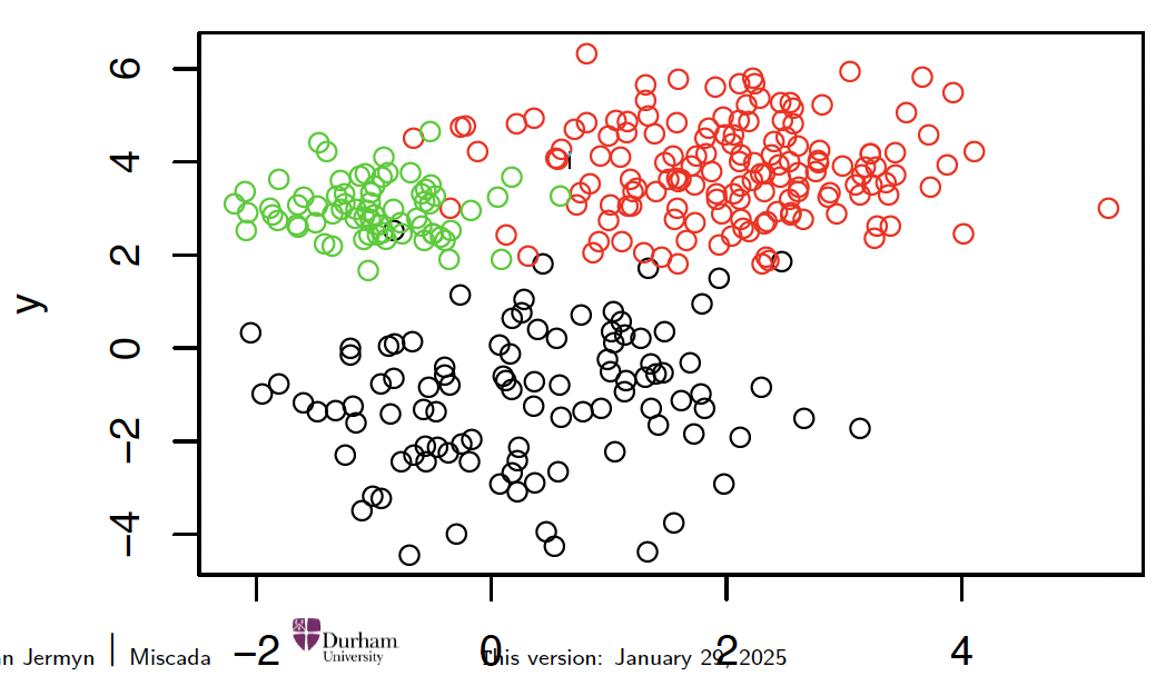
Take the simulated data with known training labels:

intro.dat <- read.table(
  "http://www.maths.dur.ac.uk/~dma0je/Data/intro-asml2.dat",
  header=TRUE
)
intro.labels <- read.table("http://www.maths.dur.ac.uk/~dma0je/Data/intro-asml2-labels.dat", header=TRUE)$x

plot(intro.dat, col=intro.labels)

k3 <kmeans(intro.dat, centers=3)

require(fossil)
rand.index(intro.labels, k3$cluster)
# [1] 0.9274491

require(mixtools)
intro.mix <mvnormalmixEM(intro.dat , k=3)
intro.cluster <apply(intro.mix$posterior, 1, which.max)
rand.index(intro.labels, intro.cluster)
# [1] 0.9538989

The clustering based on the mixture model yields a higher similarity to the true labels than the k-means result (this is not surprising since this data set was generated from a Gaussian mixture!)

One can also compare the similarity of two clustering outcomes:

rand.index(k3$cluster, intro.cluster)
[1] 0.9328762

‘Chance-corrected’ version: Adjusted Rand index (not further discussed here; available in mclust).

Practical 3

In the third lab session (fetch Practical 3 on Jupyter), we will:

• look into a detailed ‘case study’ illustrating how to use cluster analysis for image segmentation;
• learn how to ‘open’ an image in R and prepare it for further analysis;
• explain how the problem of segmentation relates to the question of clustering;
• explain how different clustering techniques can be used to address this problem.