[[2025-01-23-UL-2]]

UL Part 4: Dimensionality Reduction

Overview over Part 4

We will…

• derive ‘principal components’, and show how they relate to variance decomposition;
• illustrate how principal components can be interpreted and applied;
• connect principal components to autoencoders;
• introduce the concept of neural networks and demonstrate how neural networks can be used to build more sophisticated autoencoder.

Principal components

Example:

Data set of size $n = 8286$, simulated prior to launch of Gaia mission.

Available: photon counts in $p = 16$ wavelength bands.

(The scientific question is how to relate these spectra to certain stellar parameters such as temperature or metallicity, but this question is left for the ‘Regression’ module)

gaia <- read.table(
  "http://www.maths.dur.ac.uk/~dma0je/Data/gaia.dat",
  header=TRUE
)

Principal components

‘Pairs plot’

require(lattice)
s <sample(nrow(gaia), 200)
splom(gaia[s, 5:20],
      cex = 0.3,
      pscales = 0)

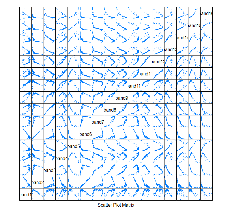
While this plot shows the individual bivariate projections, note that this is of course just one data set in 16-dimensional space.

Objective:

For a given dimension $d < 16$, approximate the data set through the ‘best’ $d$-variate linear subspace.

In the case $d = 1$:

If we were to approximate this data set through a single straight line, what would be the ‘best’ line?

Principal component analysis

The last question can be quantified as follows.

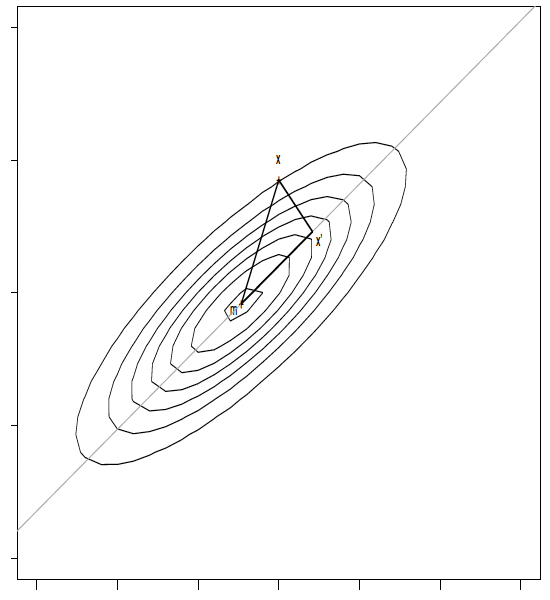
Let $X = (x_1^T, \ldots, x_n^T)^T \in \mathbb{R}^{n \times p}$ the data matrix, and $\mathbf{m} \equiv \bar{x} = \frac{1}{n} \sum_{i=1}^n x_i$ the overall mean of $X$. We would like to find a direction, in form of a unit vector $\gamma$, which defines a line, $g$,

\[g(t) = \mathbf{m} + t \gamma\]

so that the sum of squared differences between the points, $x_i$, and the projections of $x_i$ on the line, say $x’_i$, is minimal, so

\[\hat{\gamma} = \arg\min_{\gamma} \sum_{i=1}^n \| x_i - x'_i \|_2^2.\]

What is an orthogonal projection?

Mathematically,

\[x_i' = m + \gamma \gamma^T (x_i - m)\]

One can easily verify that then

\[(x_i' - m)^T (x_i' - x_i) = 0\]

so that the projection is indeed orthogonal.

Minimization squared distances = Maximizing variance

From Pythagoras, one has

\[\|x_i - x'_i\|^2 = \|x_i - m\|^2_2 - \|x'_i - m\|^2_2,\]

so that minimizing (w.r.t. γ)

\[\sum_{i=1}^n \|x_i - x'_i\|^2\]

is equivalent to maximizing

\[\sum_{i=1}^n \|x'_i - m\|^2_2.\]

Maximizing variance of projected points

Observe that

\[\begin{aligned} |\boldsymbol{\gamma}^T(\boldsymbol{x}_i-\boldsymbol{m})| & \begin{array} {rcl}= & ||\boldsymbol{\gamma}||_2\left||\boldsymbol{x}_i-\boldsymbol{m}||_2\right.|\cos(\gamma,\boldsymbol{x}_i-\boldsymbol{m})| \end{array} \\ & \begin{array} {rcl}= & ||x_i-\boldsymbol{m}||_2\frac{||x_i^{\prime}-\boldsymbol{m}||_2}{||x_i-\boldsymbol{m}||_2}=||x_i^{\prime}-\boldsymbol{m}||_2 \end{array} \end{aligned}\]

so that we want to maximize

\[\frac{1}{n} \sum_{i=1}^{n} ||x'_i - m||^2_2 = \frac{1}{n} \sum_{i=1}^{n} \gamma^T (x_i - m)(x_i - m)^T \gamma = \gamma^T \Sigma \gamma\]

where

\[\Sigma = \frac{1}{n} \sum_{i=1}^{n} (x_i - m)(x_i - m)^T\]

is the estimated variance matrix of $X$.

Hence, what remains is to maximize $\gamma^T \Sigma \gamma$ under the constraint $|\gamma|^2_2 = 1$. This is a constrained optimization problem; mathematically this is dealt with through a Lagrange multiplier, by maximizing

\[P(\gamma) = \gamma^T \Sigma \gamma - \lambda (\gamma^T \gamma - 1). \tag{1}\]

One can show that any solution of (1) fulfills

\[\Sigma \gamma = \lambda \gamma \tag{2}\]

that is $\gamma$ must be an eigenvector of $\Sigma$.

$\Sigma$ is a symmetric matrix so all its p eigenvectors are orthogonal. Let us order the eigenvalues by $\lambda_1\geq\ldots\geq\lambda_p$ with associated eigenvectors $\gamma_1,\ldots,\gamma_p$.

Now, which of these corresponds to the first principal component?

Multiply (2) from the left with $\gamma^T$:

\[\gamma^T\boldsymbol{\Sigma}\gamma=\lambda\gamma^T\boldsymbol{\gamma}(=\lambda)\quad(3)\]

The left hand side of this is just what we want to maximize!

So, the direction of the first principal component is given by the eigenvector $\gamma_1$ corresponding to the largest eigenvalue, $\lambda_1$.

The k-th principal component

We call the new coordinates defined by $\gamma^T_1(x_i - m)$ the first principal component scores and the line $g_1(t) = m + t\gamma_1$ the first principal component line.

Similarly, the k-th principal component scores are defined by $\gamma^T_k(x_i - m)$, with k-th principal component line

\[g_k(t) = m + t\gamma_k\]

This is the line through $m$ which minimizes the sum of squared distances to the data among all lines which are orthogonal to $\gamma_1, \ldots, \gamma_{k-1}$.

[H Sec 14.5.1, J Sec 10.2]

PCA for Gaia data

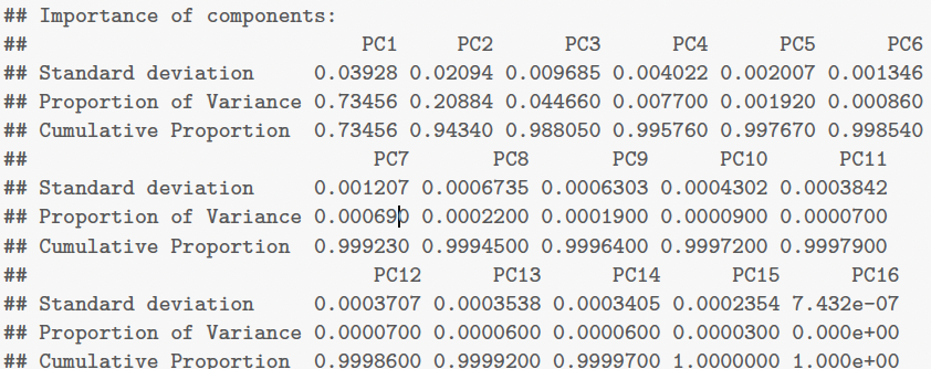
gaia.pr <prcomp(gaia[,5:20])
gaia.pr$sdev

## [1] 3.927884e-02 2.094376e-02 9.684892e-03 4.021731e-03 2.007252e-03
## [6] 1.345609e-03 1.207150e-03 6.735267e-04 6.302979e-04 4.301512e-04
## [11] 3.842127e-04 3.707281e-04 3.538154e-04 3.404939e-04 2.353966e-04
## [16] 7.432292e-07

These are just the square roots of the eigenvalues $\lambda_j$. So, we obtain the $\lambda_j$ as

Lambda <gaia.pr$sdev^2
round(Lambda, digits=6)

## [1] 0.001543 0.000439 0.000094 0.000016 0.000004 0.000002 0.000001 0.000000

## [9] 0.000000 0.000000 0.000000 0.000000 0.000000 0.000000 0.000000 0.000000 0.000000

and, more usefully,

round(Lambda/sum(Lambda), digits=3)

## [1] 0.735 0.209 0.045 0.008 0.002 0.001 0.001 0.000 0.000 0.000 0.000 0.000
## [13] 0.000 0.000 0.000 0.000

which is just the proportion of ‘total’ variance explained by the jth principal component.

One can also find this information from

summary(gaia.pr)

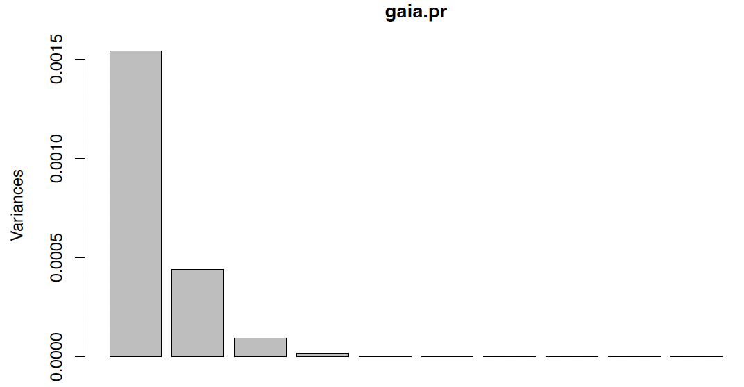
Scree plot

The most common way to graphically represent this information is a scree plot [J Sec 10.2.3].

plot(gaia.pr)

How many principal components?

We have learned how a data set can be compressed onto an adequate $k$-dimensional subspace. The dimension $k$ can be selected through different means, for instance by

• identifying the kink in a scree plot
• select as many principal components as needed in order to explain a given proportion, say 95%, of the original variation.

For the Gaia data, both criteria would suggest $k = 3$. This captures almost 99% of the variation in the data.

Ocean data

4-dimensional ocean data¹:

ocean <- read.table(
  "http://www.maths.dur.ac.uk/~dmaOje/Data/ocean.dat",
  header=TRUE, sep=","
)
pairs(ocean)

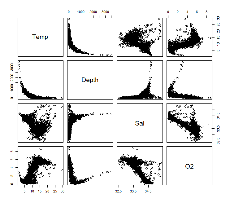
¹ subset of much larger data set, extracted from https://www.kaggle.com/sohier/calcifi/

head(ocean)
##   Temp Depth     Sal   O2
## 1 11.01    75 33.099 4.99
## 2  1.78  2600 34.637 2.22
## 3 21.42    10 33.712 5.26
## 4  9.17    97 33.822 2.96
## 5  5.51   462 34.230 0.70
## 6 14.95    66 33.380 5.94

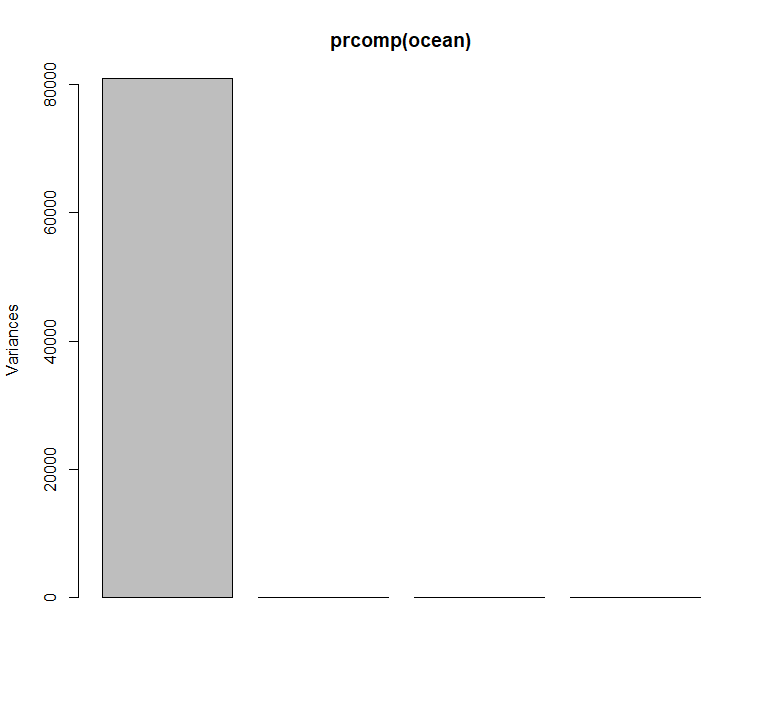
dim(ocean)
## [1] 2500    4

plot(prcomp(ocean))

Direct application of PCA useless!

Why?

Correlation matrix

All variables in the ocean data set operate on very different units. These are not comparable so their relative variances are meaningless.

var(ocean)

##       Temp       Depth        Sal         O2
## Temp  17.774113 -850.31187  -1.0359905  7.1151393
## Depth -850.311868 80833.66920 79.7817657 -394.623548
## Sal   -1.035990  79.78177   0.2125981 -0.8104315
## O2    7.115139  -394.62335 -0.8104315  4.3887447

In such cases, the variance/covariance matrix $\Sigma$ used for PCA needs to be replaced by the correlation matrix, $R$:

cor(ocean)

## Temp   Depth     Sal        O2
## Temp      1.0000000 -0.7093950 -0.5329446  0.8055997
## Depth    -0.7093950  1.0000000  0.6085942 -0.6625467
## Sal      -0.5329446  0.6085942  1.0000000 -0.8390086
## O2       0.8055997 -0.6625467 -0.8390086  1.0000000

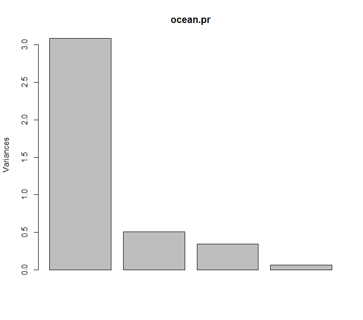
PCA with Correlation matrix

This can be easily done via

ocean.pr <prcomp(ocean, scale=TRUE)
ocean.pr$sdev^2/sum(ocean.pr$sdev^2)
## [1] 0.77132180 0.12710122 0.08573903 0.01583795

plot(ocean.pr)

Interpretation of principal components

ocean.pr

## Standard deviations (1, ..., p=4):
## [1] 1.7564986 0.7132051 0.5856246 0

# Interpretation of principal components

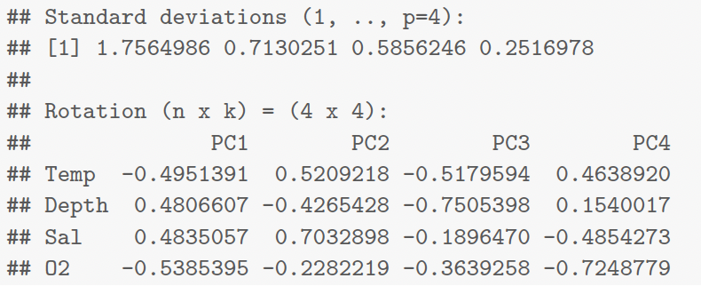
As said previously, the Standard deviations are just $\sqrt{\lambda_j},j=1,\ldots,4$. The columns of the $matrix \ Rotation\equiv\Gamma$ are just the $\gamma_j,j-1,\ldots,4$.

From the Rotation matrix, we see that

• the first principal component is large when Depth and Sal are large.

• the second principal component is large when Temp and Sal are large.

• the third principal component captures the joint trend of all variables.

• the fourth principal component is large when Sal and O2 are small.

Some more PCA properties…

• From (2) one obtains the eigen decomposition

\[\Sigma=\Gamma\Lambda\Gamma^T\]

• This can also be written as the spectral decomposition

\[\Sigma=\sum_{j=1}^p\lambda_j\gamma_j\gamma_j^T\]

• From the eigen decomposition, one can derive

\(\left.\mathsf{Cov}(\gamma_j^T(\boldsymbol{X}^T-\boldsymbol{m}),\boldsymbol{\gamma}_k^T(\boldsymbol{X}^T-\boldsymbol{m}))=\left\{ \begin{array} {cc}0 & j\neq k \\ \lambda_j & j=k \end{array}\right.\right.\) In particular, principal component scores corresponding to different eigenvectors are uncorrelated variables.

PC scores for ocean data

Principal component scores can be thought of the coordinate of the ith observation in a coordinate system centered at $m$, where the axes span the directions of the principal components. Their values, $\gamma_j^T (x_i - m)$, are given in the ith row and jth column of the following matrix.

head(ocean.pr$x)
##       PC1         PC2        PC3        PC4
## [1,] -1.4253991 -1.0510422 0.3886722 0.15349986
## [2,]  6.2522645 -3.3319874 -5.2943427 -0.15514495
## [3,] -2.1844861  1.23832989 -1.0177201 0.52494668
## [4,]  0.1078985  0.01253955 0.6119242 -0.09580616
## [5,]  2.1636308 -0.11875991 0.3228286 0.05163269
## [6,] -1.8528960 -0.22559704 -0.3522365 -0.04239513

Independence of PC scores for ocean data

round(var(ocean.pr$x), digits=4)

	PC1	PC2	PC3	PC4
PC1	3.0853	0.0000	0.0000	0.0000
PC2	0.0000	0.5084	0.0000	0.0000
PC3	0.0000	0.0000	0.3430	0.0000
PC4	0.0000	0.0000	0.0000	0.0634

round(cor(ocean.pr$x), digits=4)

	PC1	PC2	PC3	PC4
PC1	1	0	0	0
PC2	0	1	0	0
PC3	0	0	1	0
PC4	0	0	0	1

Compression-Reconstruction view of PCA

Projecting (‘compressing’) all data points $x_i, i = 1, \ldots, n$ onto the $d$−dim. subspace spanned by the $d$ largest principal components

\[f : \mathbb{R}^q \to \mathbb{R}^d, \quad x_i \mapsto (\gamma_1, \ldots, \gamma_d)^T (x_i - m), \quad i = 1, \ldots, n\]

and mapping back (‘decompressing’) the scores $f(x_i) \equiv t_i$ to the data space

\[g : \mathbb{R}^d \to \mathbb{R}^q, \quad t_i \mapsto m + (\gamma_1, \ldots, \gamma_d)t_i, \quad i = 1, \ldots, n\]

gives ‘reconstructed’ values $r_i \equiv (g \circ f)(x_i)$.

The original data will not be exactly reconstructed (as we have dismissed some information), unless $d = p$.

Why do PCA?

• Compression of high-dimensional data sets (storage, transportation, computation time);
• Preparation for further processing:
  • Regression (reduced-dimensional predictor space using scores of leading principal components, see ‘Regression” submodule),
  • Classification (such as digit recognition, see Lab 4);
• Denoising (images etc).

Autoencoders

• PCA can be interpreted as a compression/reconstruction algorithm, also known as an encoder/decoder:

  \[r_i \equiv (g \circ f)(x_i)\]

• Its simplicity (its linearity) might limit its applicability.

• Can we learn more expressive non-linear functions for the encoder, $f$, and decoder, $g$?

• Neural networks provide such functions, but we can no longer derive the optimal solution analytically. We need another approach…

Crash course: Neural Networks

• Recall basic linear regression:

  \[\hat{y} = h(\mathbf x, \theta) = \mathbf Wx + \mathbf b,\]

  with $\theta = (\mathbf W, \mathbf b).$

• We can make the model more flexible by using data transformations such as polynomials $\phi(\mathbf x) = (\mathbf x, \mathbf x^2, \mathbf x^3, \ldots)$

  \[h(\mathbf x, \theta) = \mathbf W\phi(x) + \mathbf b.\]

• Limitation: we need to think of reasonable functions $\phi$ that make sense with the data at hand.

• Perhaps learn feature extractions

  \[h(\mathbf x, \theta) = \mathbf W_1 \phi(\mathbf W_2 x + \mathbf b_2) + \mathbf b_1\]

  for some function $\phi$.

• $\phi$ should not be a linear function because \(h(\mathbf{x},\theta)=\mathbf{W}_1(\mathbf{W}_2\mathbf{x}+\mathbf{b}_2)+\mathbf{b}_1=\underbrace{\mathbf{W}_1\mathbf{W}_2}_{=\mathbf{W}}\mathbf{x}+\underbrace{\mathbf{W}_1\mathbf{b}_2+\mathbf{b}_1}_{=\mathbf{b}}.\)

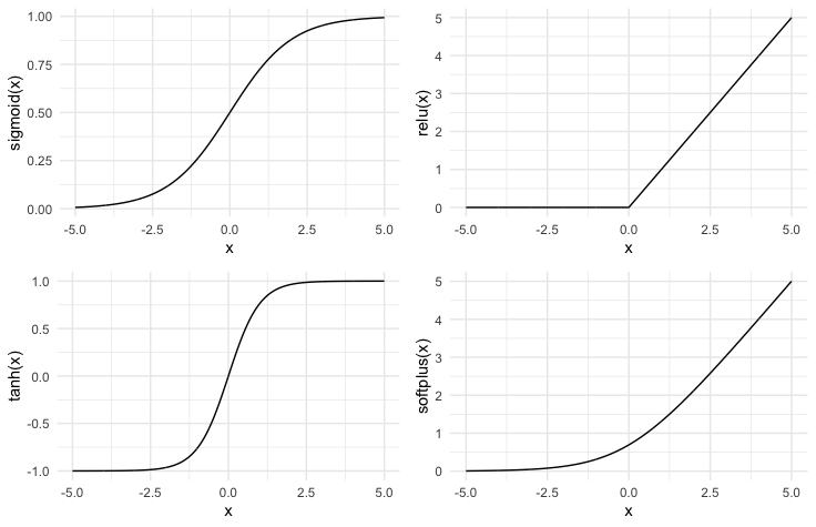
Activation functions

We need to choose some non-linear function $\phi$ to learn non-linear features. Typical choices:

• sigmoid$(x) = \frac{1}{1+e^{-x}}$
• relu $(x) = max(0, x)$
• tanh$(x)$
• softplus$(x) = log(1 + e^{x})$

2-Layer Neural Network

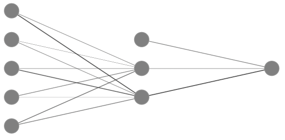
Take activation function $\sigma$,

\[z_1 = w_{11}x_1 + w_{12}x_2 + w_{13}x_3 + w_{14}x_4 + b_{11}\] \[z_2 = w_{21}x_1 + w_{22}x_2 + w_{23}x_3 + w_{24}x_4 + b_{12}\] \[\text{output} = w_1\sigma(z_1) + w_2\sigma(z_2) + b_1\]

Deep Learning

• Two-layer (one hidden layer) neural network are ‘universal approximators’, i.e. they can approximate any continuous function arbitrarily well for large enough layer width.

• However, we can iterate the nesting approach above

  \[h(x, \theta) = W_1\sigma(W_2\sigma(W_3\sigma(\cdots) + b_3) + b_2) + b_1,\]

  where $\theta = (W_1, b_1, W_2, b_2, \ldots)$

• Hence, every layer can make use of the features constructed in previous layers. This facilitates the construction of very complex features.

Loss Function

• Given some data $(y_i, x_i)$, $i = 1, \ldots, n$, the task is defined by a loss function

\[\mathcal{L}(y, x, \theta) = \sum_{i=1}^{n} \ell(y_i, x_i, \theta).\]

• Can usually be interpreted as a log-likelihood (cf Foundations).

• For binary classification, we can use the cross-entropy log-likelihood:

\[\sum_{i} y_i \ln (\sigma(h(x_i, \theta))) + (1 - y_i) \ln (1 - \sigma(h(x_i, \theta))) .\]

Optimization

• In stark contrast to previous approaches, we cannot hope to find an analytic solution for the parameters θ that minimize this loss function.

• Typical numerical optimization schemes for such cases use gradient-based approaches (e.g. Newton, BFGS, gradient-descent, etc.).

• Still leaves the problem of finding gradients of h(x, θ) w.r.t. θ = (W₁, b₁, W₂, b₂, …).

• Cumbersome and not scalable.

Automatic differentiation

• Modern deep learning libraries such as pytorch and TensorFlow support automatic differentiation.

• Idea: computer code is just a concatenation of elementary functions with known derivatives. If we keep track of the functions we can automatically compute the gradients using the chain rule.

⇒ No need to worry about gradients, automatically taken care of by software.

Gradient-descent

• Recall, we want to find a stationary point $θ^*$ such that
  \(\nabla\mathcal{L}(\mathbf{y},\mathbf{x},\theta^*)=0.\)

• Gradient descent methods iteratively update a candidate $θ_0$
  \(\theta_{i+1}=\theta_i-\eta\cdot\nabla\mathcal{L}(\mathbf{y},\mathbf{x},\theta_i).\)

Here η is called the learning rate and controls how fast the algorithm moves towards the stationary point. A too-large choice, however, will prevent convergence.

Gradient-descent

Run this code in R to get a nice animation of gradient descent:

require("animation")
grad.desc(function(x, y) 3*x + x^2 + 5*y^2,
           rg = c(-5, -3, 1, 3),
           col.contour="grey50",
           col.arrow="dodgerblue4")

Stochastic Gradient-descent

• Data sets can be very large, with billions of data points. It is often convenient to only use a subset of data every iteration.

• It is also useful: the use of partial data introduces ‘noise’, which helps to avoid local minima.

• Divide data into batches ${B_k}_{k \in [1..K]}$, and then iterate through them, taking one gradient step for each $k$:

  \[\theta_{i+1} = \theta_i - \frac{\eta}{|B_k|} \cdot \sum_{i \in B_k} \nabla \ell(y_i, x_i, \theta_i).\]

• One pass through the whole data set is called an epoch.

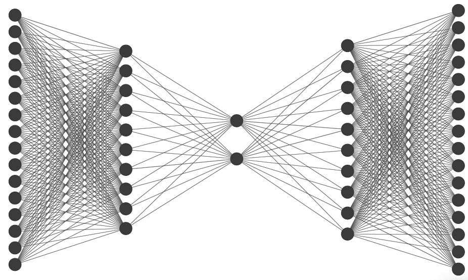
Bottleneck Autoencoders

• Recall the encoder/decoder interpretation of PCA:

  \[r_i \equiv (g \circ f)(x_i)\]

  Now let’s parameterize $f$ and $g$ with neural networks.

• Input and output are identical, but all information is ‘squeezed’ through a bottleneck, i.e. mapped to a lower-dimensional space, à la PCA, but nonlinear.

• As loss function, use, for example, mean squared error:

  \[\mathcal{L}(x, \theta) = \sum_{i=1}^{n} \|x_i - (g \circ f)(x_i)\|^2\]

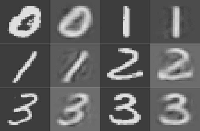
Bottleneck Autoencoders

require(rsrd)
data(digits)

digits.dat <digits[,2:785]/255
rownames(digits.dat) <digits[,1]
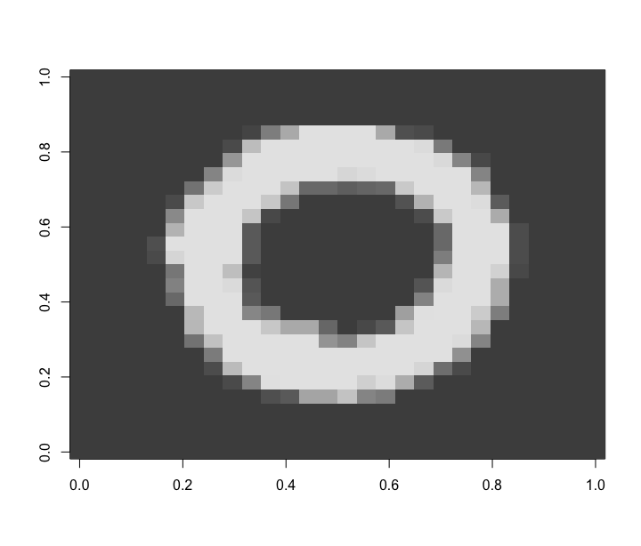
image(matrix(digits.dat[1, , drop=FALSE], 28, 28), col=grey.colors(100))

require("ANN2")
AE <autoencoder(digits.dat, c(400, 200, 20, 200, 400),
                  loss.type = 'squared',
                  activ.functions = c('tanh', 'tanh', 'sigmoid', 'tanh', 'tanh'),
                  batch.size = 256, optim.type = 'sgd',
                  n.epochs = 100, val.prop = 0.1)

recX <reconstruct(AE, digits.dat[2000*1:6, ])
par(mfrow=c(3, 4), mai=rep(0, 4))
for(i in 1:6) {
  image(matrix(digits.dat[2000*i, ], 28, 28)[,28:1],
        col = grey.colors(255), axes=FALSE)
  image(matrix(recX$reconstructed[i, ], 28, 28)[,28:1],
        col = grey.colors(255), axes=FALSE)
}

Practical 4

In the final lab session (fetch Practical 4 on Jupyter), we will:

• consider a complex data set involving handwritten digits from the MNIST data base
• use principal components to compress handwritten digits
• understand how principal component scores can be used for digit recognition purposes;
• reconstruct digits based on a set of principal component scores.