UP-L1
Part 1: Basics of multivariate analysis
First: What is learning?
- Learning means finding probability distributions to model data $Y$.
- 概率分布对数据建模
- We will see many examples of this Foundations:
Estimating the parameters $a$ of a parametric model $P(Y a)$.
- So we will know how to learning.
Supervised Learning 监督式学习
- Special case of learning.
- ‘Supervised’ means that data comes in pairs: 成对
- In addition to $Y$ there are conditioning variables $X$.
The task is to $P(Y X)$.
- Essentially the same framework as ‘conditional models’ from Foundations, so we will know how to do that too.
- What about ‘unsupervised’?
Unsupervised Learning 无监督学习
- Special case of learning. (Again)
- ‘Unsupervised’ means one of two things:
- The distribution does not depend on $X$.
- 分布不依赖 X
- We simply do not know the corresponding $X$ values.
- X值是未知的
- The distribution does not depend on $X$.
- Case 1 seems straightforward: there is no $X$.
Case 2 seems impossible: $X$ could be anything!

- Both these things are true, so why do we have this submodule?!
… contd
An outline of ASML (UL)
Part 1: Basics of multivariate analysis (ca. 3 Lectures)
- k-means
- variance matrix
- multivariate normal distribution
Part 2: Density estimation (ca. 3 Lectures)
- Gaussian mixtures
- kernel density estimation
Part 3: Cluster analysis (ca. 3 Lectures)
- Mixtureand -density based clustering
- assessing goodness of fit
Part 4: Dimensionality Reduction (ca. 3 Lectures)
- Principal component analysis and (deep) autoencoders.
Part 1: Basics of multivariate analysis
多变量分析基础知识
Overview over the remainder of Part 1
We will…
- look in detail into k-means (firstly conceptually, then based on the notion of dissimilarities); as well as some variants including k-medoids;
- discuss the estimation of mean, variance, and correlation matrix of a random vector;
- recall the normal distribution, and introduce the multivariate normal distribution;
- define Mahalanobis distances (another dissimilarity) and use them to check for outliers and multivariate normality.
K-means clustering
Probably the most famous clustering technique.
Objective: For a fixed number of clusters集群, find a set of clusters which minimizes the sum of squared distances between data and their cluster centres (to be formalized later).
This is a special case of Gaussian mixtures, which we will study later in the course.
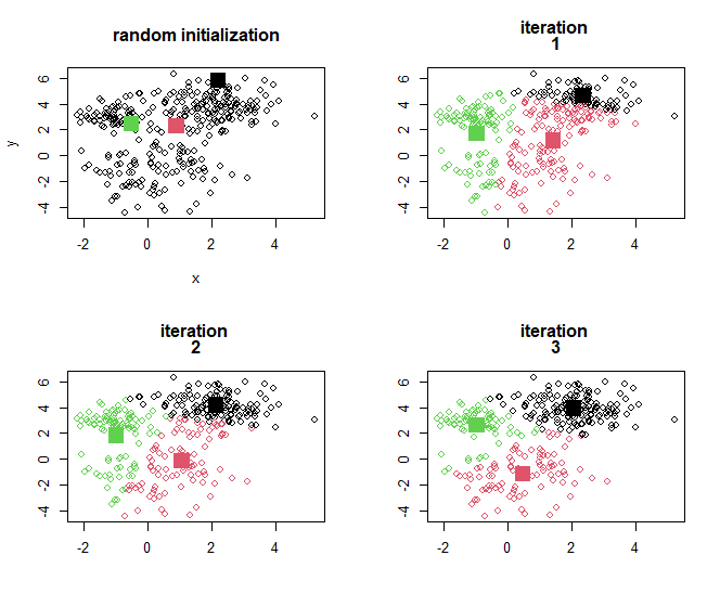
One can show that a local minimum of this objective is achieved by the following algorithm. For a data set with ( n ) observations:
Select the number of classes, ( K ), in advance.
Randomly select ( K ) out of the ( n ) cases as initial cluster centres.
Then repeat
(i) Assign all observation to their nearest centre (producing a partition in ( K ) parts)
(ii) Compute the mean of each partition, producing updated centres
… until the centres stop moving.
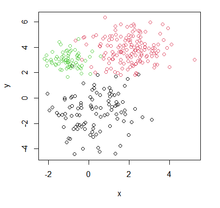
Illustration: K-means
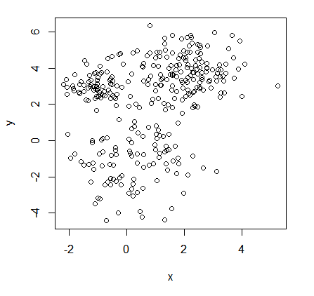
Consider again the unlabelled data set illustrated previously.
Set $K = 3$ (subjective choice by data analyst, expert knowledge,…).
Analysis in R: Reading in data
1
2
3
4
5
6
7
8
9
10
11
12
13
14
intro.dat <- read.table(
  "http://www.maths.dur.ac.uk/~dma0je/Data/intro-asml2.dat",
  header=TRUE
)

head(intro.dat)

##      x          y
## 1 -0.4720543 -1.3495412
## 2 -2.0489395  0.3468624
## 3 -1.3263892 -1.3380228
## 4  1.7823161 -0.9631754
## 5  0.5540121  0.2210657
## 6 -0.8238523  0.1000506
K-means in R
1
2
3
4
5
6
7
8
9
10
11
k3 <kmeans(intro.dat, centers=3)
k3$centers

##      x          y
## 1 0.2621725 -1.267684
## 2 -0.8169763  2.996031
## 3 2.1752499  3.826271

k3$cluster[1:20]

##  [1] 1 1 1 1 1 1 1 1 1 1 1 1 1 1 1 1 1 1 1 1
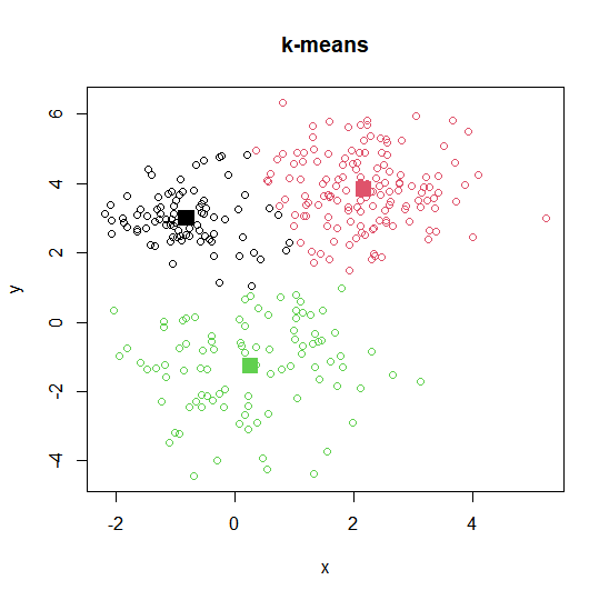
Plotting k-means output
1
2
3
plot(intro.dat, col=k3$cluster, main="k-means")

points(k3$centwes, pch=15, cex=2, col=c(1, 2, 3))
Dissmilarity 差异性
- 组件级(Component-wise)差异性
- 常见损失函数
- 组合多个属性的差异性
- 欧几里得距离(Squared Euclidean Distance)
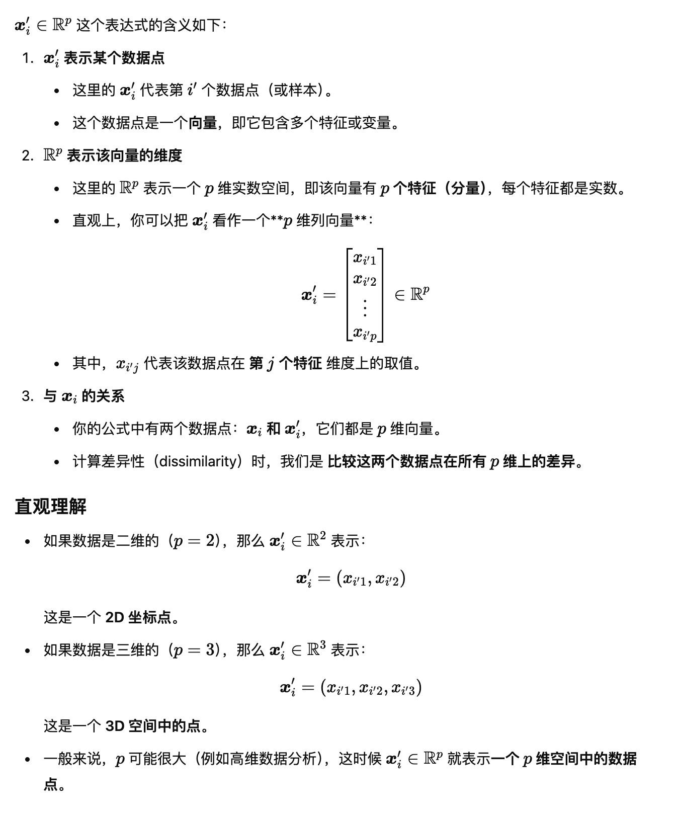
To understand on a deeper level what $k$-means is trying to achieve, one needs to introduce the concept of a dissimilarity, $D(x_i,x_i’)$ between two points $x_i$ and $\boldsymbol{x}_i^{\prime}\in\mathbb{R}^p$.
$x$和$x’$就是两个不同的数据点。
Often, these dissimilarities are defined component-wise (按组件定义), based on dissimilarity measures between the the values of the $j$th variable (attribute),
\[d_j(x_{ij},x_{i^{\prime}j})=\ell(x_{ij}-x_{i^{\prime}j})\]with a loss function $l(\cdot)$ ; for instance, 损失函数
- $d_j(x_{ij},x_{i^{\prime}j})$ 第$j$个变量(属性)的差异性度量
- $l(\cdot)$ 损失函数
- $\ell(z)=z^2$ (squared error loss); 平方误差损失
$\ell(z)= z $ (absolute loss). 绝对损失
The $p$ attribute-wise dissimilarities can be merged into a single overall measure of dissimilarity between objects $i$ and $i’$ via
- 属性上 不相似性
where $w_j$ is a set of weights. 权重 Simple example: Set $l(z)=z^2$ and $w_j=(1,…,1)$. Then
\[D(\boldsymbol{x}_i,\boldsymbol{x}_i^{\prime})=\sum_{i=1}^n(x_{ij}-x_{i^{\prime}j})^2=||\boldsymbol{x}_i-\boldsymbol{x}_i^{\prime}||^2=(\boldsymbol{x}_i-\boldsymbol{x}_i^{\prime})^T(\boldsymbol{x}_i-\boldsymbol{x}_i^{\prime}).\](squared Euclidean distance 欧几里得距离)
Dissmilarity and k-means
K-Means 聚类算法的核心是 基于“差异性”(Dissimilarity)最小化簇内平方和(Within-cluster Sum of Squares, WSS)。 Note firstly that, for a collection of data $x_1, . . . , x_n$, one can describe the iterative part of the k-means algorithm entirely through two optimization steps rooted in dissimilarities:
- 两个迭代优化步骤
(i) For a given set of cluster centres, say $c_k$, $k = 1 . . . ,K$, assign each observation $x_i$to partition分区 $C_k$, with k given by
- 分配到最近的簇
(ii) For a given partition $C_1, . . . ,C_K$, find the updated centre via
- 在一个数据点被分配到簇后,更新簇中心点
If $D$ is the squared Euclidean distance(欧几里得平方), one can show that the $k$-means algorithm finds a minimum of the within-cluster sum of squares
\[SS_{\text{within}} = \sum_{k=1}^{K} \frac{1}{n_k} \sum_{(i,\ell): i<\ell, x_i,x_\ell\in C_k} D(x_i, x_\ell) = \sum_{k=1}^{K} \sum_{i: x_i\in C_k} D(x_i, c_k)\]where $n_k$ is the number of observations in partition $k$.
- n是分区k中观测值的个数
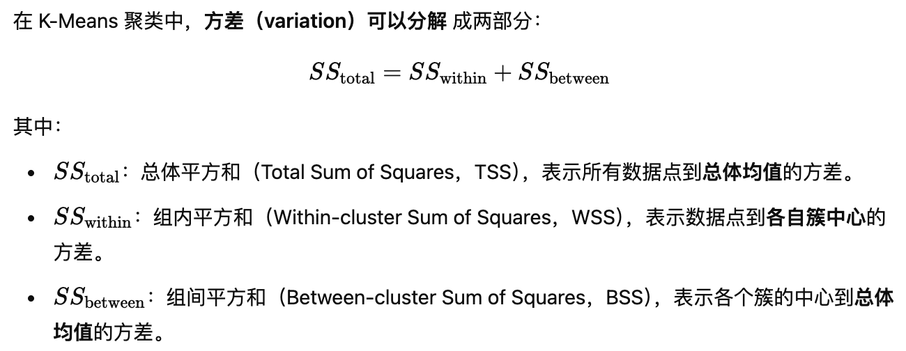
This value can be compared to the total sum of squares, 比较方式-平方和
\[SS_{\text{total}} = \sum_{i=1}^{n} \|x_i - \bar{x}\|^2 = \sum_{i=1}^{n} D(x_i, \bar{x})\]and their difference, $SS_{\text{total}} - SS_{\text{within}}$ corresponds to the between-cluster sum of squares. 聚类间平房和
Decomposing variation 变异分解
1
2
3
4
5
6
7
8
9
10
11
12
13
14
15
16
# 三个值的代码
k3$withinss  # 各簇的 SS_within(组内平方和)

## [1] 270.39234 89.49661 258.54463

k3$tot.withinss  # SS_within 总和

## [1] 618.4336

k3$totss  # SS_total

## [1] 2681.893

k3$betweenss  # SS_between

## [1] 2063.459
Sum of squares: 2681.893 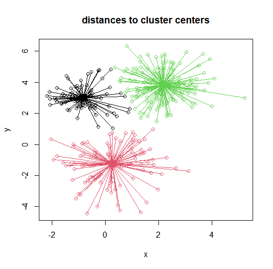
Sum of squares: 618.4336
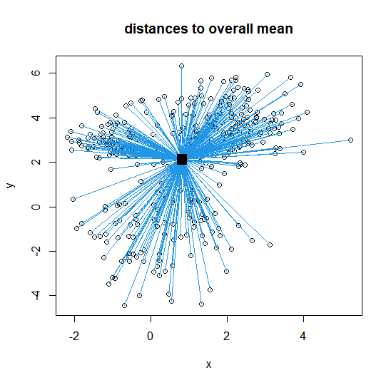
Analysis in R: Visualize projections
可视化数据点与中心的距离 Total
1
2
3
4
5
6
7
8
9
10
11
12
13
14
m <- colMeans(intro.dat)   # 计算所有数据点的总体均值(overall mean)
plot(intro.dat,
     main="distances to
     overall mean")
points(m[1] , m[2], pch=15,
       cex=2, col=1)       # 用方形标记绘制总体均值

n<-dim(intro.dat)[1]       # 获取数据点个数
for (j in 1:n){
  segments(intro.dat[j,1],
           intro.dat[j,2],
           m[1], m[2], col=4)
           # 画线连接每个数据点到总体均值
}
Cluster-wise 簇内距离可视化
1
2
3
4
5
6
7
8
9
10
11
12
13
plot(intro.dat, col=k3$cluster,          # 绘制数据点,按簇着色
     main="distances to
     cluster centres")
points(k3$centers, pch=15,
       cex=2, col=c(1,2,3))              # 绘制簇中心

for (j in 1:n){
  segments(intro.dat[j,1],
           intro.dat[j,2],
           k3$centers[k3$cluster[j],1],
           k3$centers[k3$cluster[j],2],
           col=k3$cluster[j])            # 画线连接每个数据点到其所属簇的中心
}
k-Means, chickens, and eggs
Note that k-means is a chicken-and-egg problem…. 一个先有鸡还是先有蛋的问题……
maybe就不需要过分纠结啦
- Determining the partitions requires knowing the means
- Finding the means requires knowing the partitions
- How to get started is a rather arbitrary decision!
k-Means: not a unique technique
诸多变体版本 There do exist many similar k-means algorithms, some of which differ in how this initialization step is handled, and some in other aspects:
The algorithm provided on slide 12 is Lloyd-Forgy’s algorithm (Lloyd 1957, published 1982; independently by Forgy, 1965).
Alternative: Random partitioning: First, randomly assign a cluster label to each observation, and then find the mean of these clusters. (Excellent illustration in [J Sec 10.3.1]).
Default option in R: Hartigan-Wong algorithm. Initialization as in random partitioning, but then steps (i) and (ii) are iterated point-by-point rather than for the whole data set at once [H Sec 14.3.6.].
Whether any of these variants find the global minimum of the total within-cluster sum of squares, will depend on the seed (Try!):
不同 K-Means 算法的聚类结果和计算性能比较
1
2
3
4
5
6
7
8
9
10
11
12
13
14
15
16
17
18
19
20
21
22
23
24
25
26
27
28
k31<- kmeans(intro.dat, centers=3, algorithm="Forgy")
k31$centers

##      x          y
## 1 -0.8169763  2.996031
## 2  0.2621725 -1.267684
## 3  2.1752499  3.826271

k31$tot.withinss
## [1] 618.4336

k3$iter
## [1] 8

k3 <- kmeans(intro.dat, centers=3, algorithm="Hartigan-Wong")
k3$centers
##      x          y
## 1  0.2621725 -1.267684
## 2 -0.8169763  2.996031
## 3  2.1752499  3.826271

k3$tot.withinss

## [1] 618.4336

k3$iter

## [1] 3
As with any algorithm that finds a local minimum, one can increase the chances of finding the global minimum for any variant by using multiple random starts; see option nstart in kmeans. 与任何找到局部最小值的算法一样,可以通过使用多个随机开始来增加找到任何变体的全局最小值的机会
k-Medoids
——变体方法
There are occasions when it is desirable that the cluster centres corresponds to actual observations (‘the most central observation of the cluster’).
簇中心->集群的最中心观测值,不允许簇中心随意移动
Recall: In ‘usual’ k-means, in step (ii), finding the $k$th cluster mean is equivalent(等同于) to minimizing $\sum_{\boldsymbol{x}{i}\in C{k}}D(\boldsymbol{x}_{i},\boldsymbol{m})$ over all possible centres $m$. k-Medoids replaces this by an optimization step which restricts the search space to the observations within the $k$-th cluster; i.e.
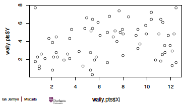
\[c_{k}^{\prime}=\mathrm{argmin}_{m\in C_{k}}\sum_{x_{i}\in C_{k}}D(\boldsymbol{x}_{i},\boldsymbol{m}).\]Example: Where’s Wally?

Data gives the locations ($X,Y$ coordinates) of where Wally (called Waldo in the US) was found in $n = 68$ double-paged illustrations in a total of seven ‘Where’s Wally’ books.
1
2
3
wally.pts = read.csv('http://www.randalolson.com/wp-content/uploads/wheres-waldo-locations.csv')

plot(wally.pts$X, wally.pts$Y) # 散点图
1
2
3
4
5
6
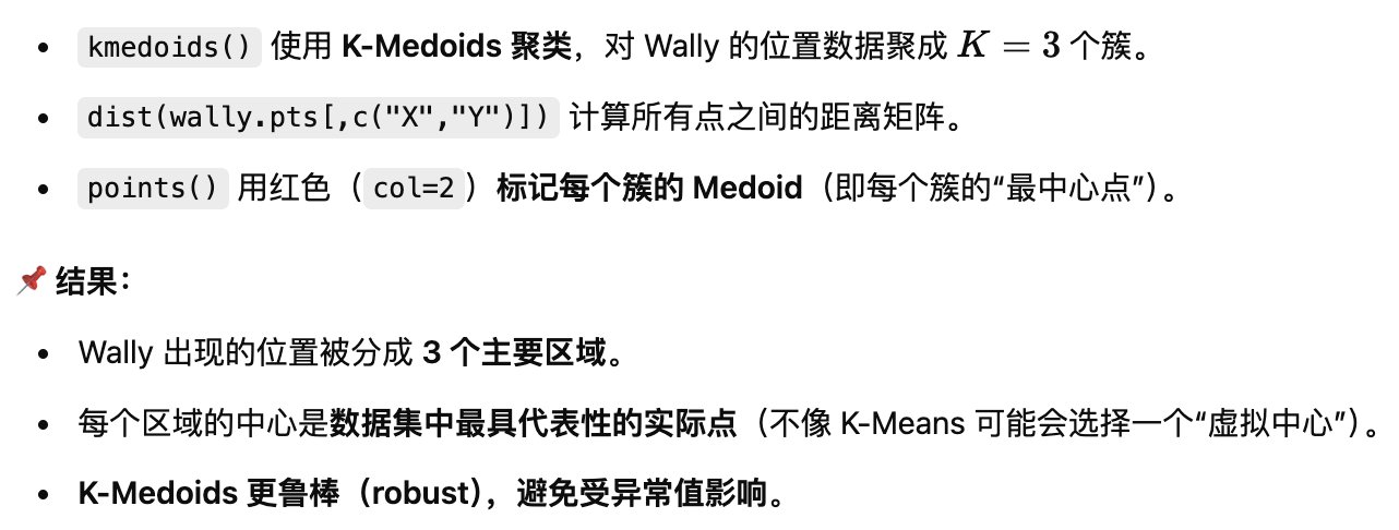
library(clue)
wally.kmed<- kmedoids(dist(wally.pts[,c("X","Y")]), k=3)
plot(wally.pts$X, wally.pts$Y)
points(wally.pts$X[wally.kmed$medoid_ids],
wally.pts$Y[wally.kmed$medoid_ids],
col=2, pch=9, cex=1.8)
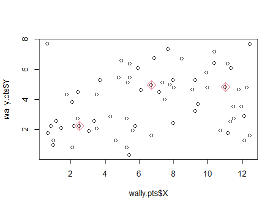 Compare to $k$-means: 对比
1
2
3
wally.kmean <- kmeans(wally.pts[,c("X","Y")], centers=3)
points(wally.kmean$centers, col=3, pch=10, cex=2)
legend(2, 8, legend=c("k-medoids", "k-means"), pch=c(9,10), col=c(2,3)) #$
- 会落在实际存在的点上
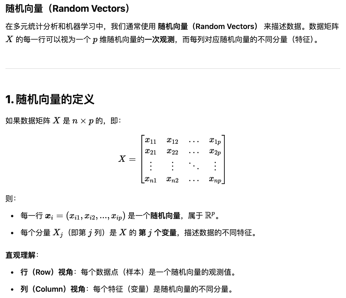
Data matrix
Let $X$ denote(表示) a data matrix (or data frame) with $n$ rows and $p$ columns (variables, features); i.e.
- 样本->矩阵
For instance, the data on slide 3 (right plot) constitute such a matrix with $( n = 320 )$ and $( p = 2 )$:
1
2
3
dim(intro.dat)

## [1] 320 2
dim() 函数返回数据集的 维度(即行数和列数)。
Random vectors
We can combine the $p$ components of each row of $X$ into a vector $X$ in $\mathbb{R}^p$. The rows of $X$ can then be thought of as realizations of a random vector, with the $j$-th component, $X_j$, being responsible for the generation of the $j$-th column of $X$.
- 每一行的分量合成向量
We have implicitly(隐式地) been using the properties of random vectors in $\mathbb{R}^2$ so far. We now make these properties more explicit and define some quantities for future use.
Properties of random vectors 随机向量的性质
概率密度函数(PDF)
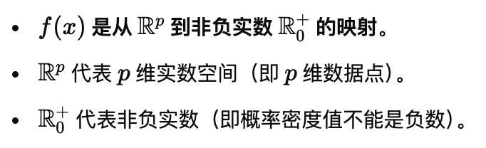
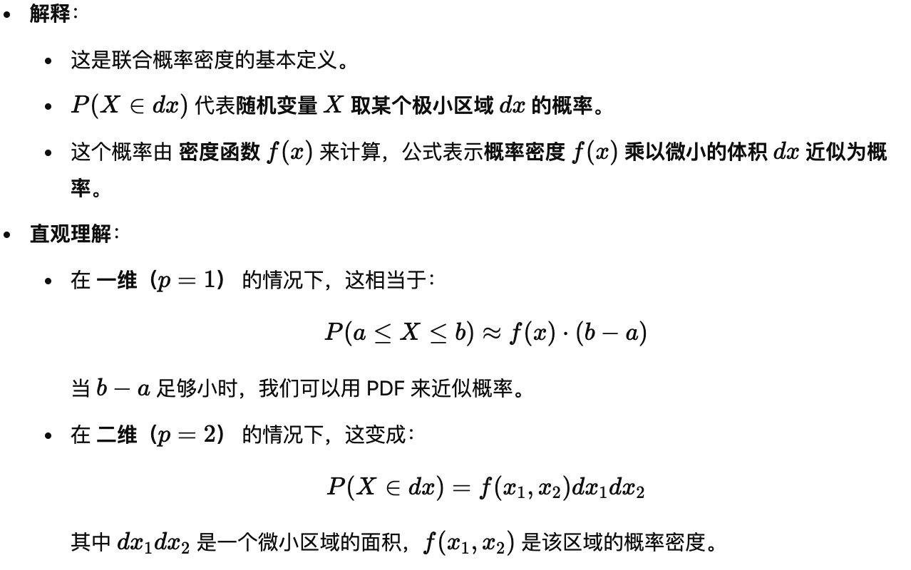
(a) There exists (under some mild conditions), a probability density function (‘density’) $f : \mathbb{R}^p \to \mathbb{R}_{0}^+$, such that
- 温和条件
- 概率密度函数
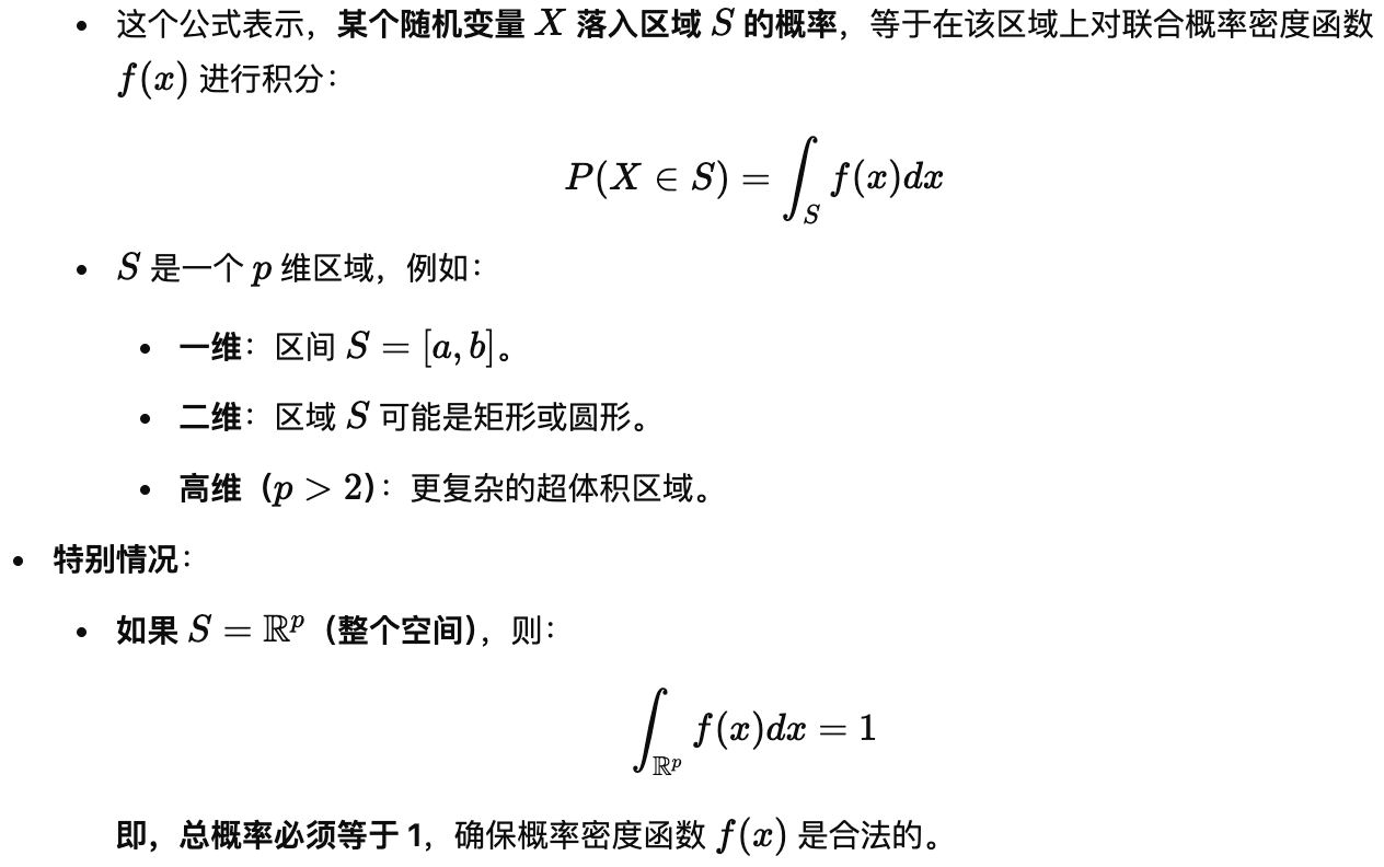
for any (appropriately well-behaved) subset $S \subset \mathbb{R}^p$. In particular, for $S = \mathbb{R}^p, \int_{\mathbb{R}^p} f(x) dx = 1$. The density $(f)$ can be estimated from data $(X)$; we deal with this problem in Part 2 of this course.
(1)  (2)
(2)
随机变量的独立性 (b) We refer to the $X_1, \ldots, X_p$ as independent if the joint density $f(x)$ can be factorized; i.e. if
- 联合概率密度
- 一个 ppp 维随机向量 $X=(X_1,X_2 \dots ,X_p )$ ,联合概率密度f
联合 PDF 是多个随机变量的概率密度函数,用来描述它们的联合分布。 - 如果他们相互独立,那么可以分解为单变量的乘积 This means that the values of any random variable $X_j$ are uninformative for the values of the other random variables.
- 独立:某个变量的值不会提供其他变量的信息
- 在实际数据分析中,大多数变量是相关的,需要计算协方差矩阵来量化这种相关性
均值向量 (c) The random vector $X$ has a mean:
\[\begin{pmatrix} m_1 \\ \vdots \\ m_p \end{pmatrix} = m = E(X) = \int x f(x) dx = \int \cdots \int \begin{pmatrix} x_1 \\ \vdots \\ x_p \end{pmatrix} f(x_1, \ldots, x_p) dx_1 \cdots dx_p\]which implies $m_j = E(X_j)$, for the $j$-th component of $m$.
- 暗示 数据的中心位置 / 均值代表变量x的期望
Estimating the mean vector 估计均值向量
Let $\mathbf{x}_i^T$ denote the $i$-th row of $\mathbf{X}$, i.e., the $i$-th observation. Then we may estimate $\mathbf{m}$ by
\[\bar{\mathbf{x}} = \frac{1}{n} \sum_{i=1}^{n} \mathbf{x}_i = \frac{1}{n} \sum_{i=1}^{n} \begin{pmatrix} x_{i1} \\ \vdots \\ x_{ip} \end{pmatrix} = \begin{pmatrix} \frac{1}{n} \sum_{i=1}^{n} x_{i1} \\ \vdots \\ \frac{1}{n} \sum_{i=1}^{n} x_{ip} \end{pmatrix} = \begin{pmatrix} \bar{x}_1 \\ \vdots \\ \bar{x}_p \end{pmatrix}\]证明估计量无偏 One can easily show that this estimator is unbiased: if we were able to draw repeated samples of size $n$ from $\mathbf{X}$, and then compute $\bar{\mathbf{x}}$ each time, the average of these estimates would tend to the true value of ${m}$ as the number of samples increased.
- 样本均值是均值向量的无偏估计**,随着样本增多,它会越来越接近真实均值 m。
- 均值向量是数据的全局特征,在数据分析中是重要的统计量。
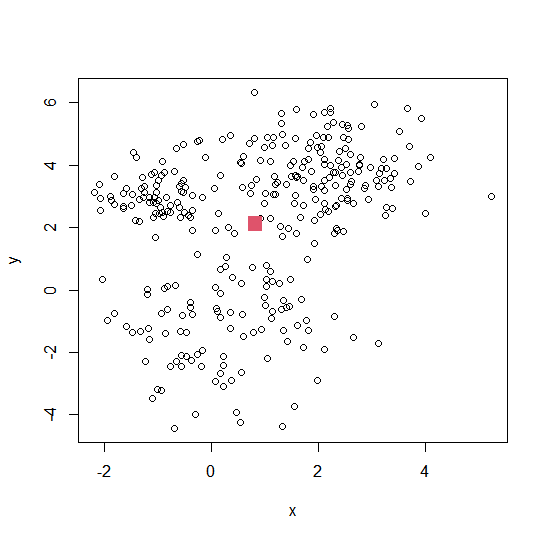
Estimating the mean vector: Example
1
2
3
m <- colMeans(intro.dat) # 计算数据矩阵的均值向量
plot(intro.dat)
points(m[1], m[2], col=2, pch=15, cex=2)  # 标记均值点
Properties of random vectors (cont’d)
在多元统计分析中,随机向量的方差矩阵(Variance Matrix)或协方差矩阵(Covariance Matrix) 描述了多个变量之间的变异性和相互关系。 (d) The random vector also possesses a variance (also called variance matrix, covariance matrix),
\[Var(X) = E((X - m)(X - m)^T) = E(XX^T) - mm^T\] \[= \begin{pmatrix} \Sigma_{11} & \cdots & \Sigma_{1p} \\ \vdots & \ddots & \vdots \\ \Sigma_{p1} & \cdots & \Sigma_{pp} \end{pmatrix} = \Sigma,\]?: 均值向量$m=E(X)$
where 对角元素和非对角元素
\[\Sigma_{ij} = Cov(X_i, X_j) = E(X_iX_j) - E(X_i)E(X_j) \quad i \neq j\] \[\Sigma_{jj} \equiv \sigma_j^2 = Var(X_j)\]Any variance matrix $\Sigma$ has the following properties:
(i) $\Sigma$ is symmetric, i.e. $\Sigma = \Sigma^T$
- 对称的 (ii) $\Sigma$ is positive semi-definite; i.e. its eigenvalues are non-negative. - 半正定的 ?什么事半正定
In short, we write
\[X \sim (m, \Sigma)\]meaning that $X$ has some unspecified distribution with mean $m$ and variance $\Sigma$. 公式没看懂
Estimating variance matrices
估计方差矩阵,它描述了数据的变异性和变量之间的关系。 Firstly, recall
\[\Sigma = \text{Var}(X) = E \left( (X - m)(X - m)^T \right).\]Replacing all expectations by means, a natural candidate estimator for $\Sigma$ is given by
\[\hat{\Sigma} = \frac{1}{n} \sum_{i=1}^{n} (x_i - \bar{x})(x_i - \bar{x})^T = \frac{1}{n} \sum_{i=1}^{n} x_ix_i^T - \bar{x}\bar{x}^T \in \mathbb{R}^{p \times p}.\]In fact, this is the Maximum Likelihood estimator for $\Sigma$ under an assumption of multivariate normality, but it is biased.
An unbiased estimator of $\Sigma$ is obtained through the sample variance matrix,
\[\hat{\Sigma} = \frac{1}{n - 1} \sum_{i=1}^{n} (x_i - \bar{x})(x_i - \bar{x})^T = \frac{n}{n - 1} \tilde{\Sigma}\]We generally prefer $\hat{\Sigma}$ to $\tilde{\Sigma}$. R functions var and cov (identical!) use this too.
In the special case of $p = 2$, $\hat{\Sigma}$ can be written as
- 二维情况
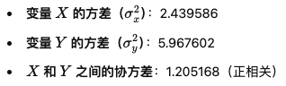
Estimating variance matrices: Example
1
2
3
4
5
6
Sigma <- var(intro.dat) # 计算样本协方差矩阵
Sigma

##         x         y
## x 2.439586 1.205168
## y 1.205168 5.967602
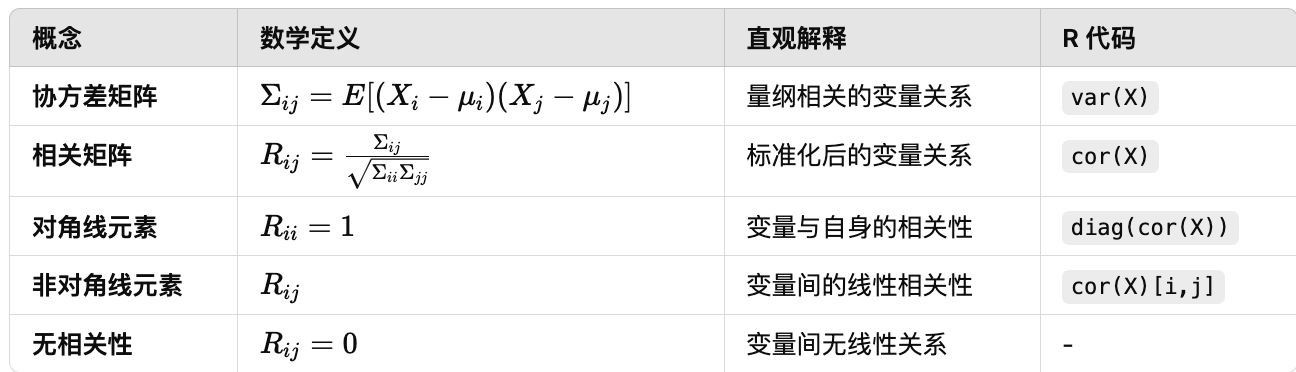
Correlation matrix
相关矩阵–标准化的协方差矩阵,用于衡量多个变量之间的线性关系。
The correlation matrix is defined as
\[\mathcal{R} = (R_{ij})_{1 \leq i \leq p, 1 \leq j \leq p}\]with pairwise correlation coefficients
- 成对相关系数
The matrix ${R}$ is scale-invariant(尺度不变), and all diagonal elements(对角元素) are equal to 1. We will use this matrix mainly for PCA (Part 4).
- $\Sigma_{ij}$,$X_i$和$X_j$的协方差
- $\Sigma_{ii}$和$\Sigma_{jj}$,$X_i$和$X_j$的方差
- 相关系数$R_{ij}$通过标准化协方差,使其在区间$[-1,1]$中,便于比较不同的尺度
We call the random variables $X_i$ and $X_j$ uncorrelated if $R_{ij} = 0$. Note:
不相关情况
- If all $X_i, i = 1, \ldots, p$ are uncorrelated then $\mathcal{R}$ becomes the identity matrix;
- 不相关 -> R为单位矩阵
- If $X_i$ and $X_j$ are independent then they are uncorrelated (but the converse does not hold).
1
2
3
4
5
6
R <- cor(intro.dat)  # 计算相关矩阵
R

##        x          y
## x 1.0000000 0.3158564
## y 0.3158564 1.0000000

The normal distribution 正态分布
A random mechanism tends to have approximately a normal (aka Gaussian) distribution if its deviation from the average is the cumulative result of many independent influences.
- 随机机制倾向于具有近似正态(又称高斯)分布,如果其偏离平均值是许多独立影响的累积结果。
Examples:
- Measurement errors;
- Minor variations in production of things (e.g. thickness of coins);
- Distribution of marks in a test (of an equally skilled cohort);
- Heights of people sampled from a population.
We will see this and other ways of justifying a Gaussian distribution in Foundations.
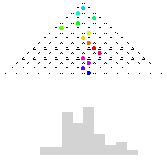
A famous tool to mimic a normal distribution is the Galton Board高尔顿板:
1
2
3
4
5
6
7
8
9
require(animation)
set.seed(42) # 设置随机种子
balls <200 # 小球数量
layers <15 # 层数
ani.options(nmax = balls + layers - 2, 2)

# 运行高尔顿板模拟
galton.sim = quincunx(balls = balls,
                       col.balls = rainbow(layers))
 Galton Board in progress.
See full animation in R! Final outcome of animation:
1
barplot(galton.sim, space = 0)
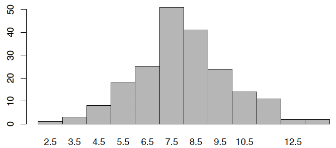
Probability density function of a (univariate) normal distribution with mean $\mu$ and variance $\sigma^2$, short $X \sim N(\mu, \sigma^2)$:
- 一元正态分布
- $\mu$ 均值
- $\sigma^2$ 方差
- $\sigma$ 标准差
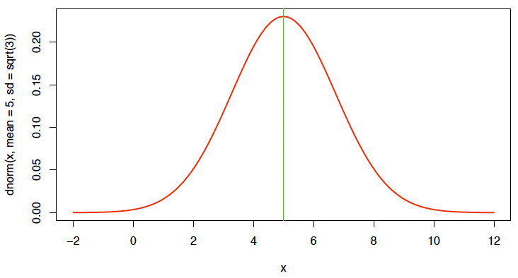
For instance, density function for $\mu = 5$ and $\sigma^2 = 3$:
1
2
3
4
x <seq(-2, 12, length=101)  # 生成 x 轴范围
plot(x, dnorm(x, mean=5, sd=sqrt(3)), type="l", lwd=2, col=2)  # 绘制正态分布
abline(v=5, col=3)  # 添加均值的竖线
“[The normal distribution] cannot be obtained by rigorous deductions. Several of its putative proofs are awful [. . .]. Nonetheless, everyone believes it, as M. Lippmann told me one day, because experimenters imagine it to be a mathematical theorem, while mathematicians imagine it to be an experimental fact.” — Henri Poincaré, Le calcul des Probabilités. 1896
Actually not true! Maximum entropy and the central limit theorem justify the Gaussian distribution.
Multivariate normal distribution 多元正态分布
多元正态分布(Multivariate Normal Distribution, MVN)是单变量正态分布的推广,用于描述多个互相关联的正态随机变量。
A random vector $X = (X_1, X_2, \ldots, X_p)^T$ is multivariate normal if (and only if) any linear combination of the random variables $X_1, X_2, \ldots, X_p$ is univariate normally distributed, i.e. iff
\[a_1X_1 + a_2X_2 + \cdots + a_pX_p\]has a univariate normal distribution(单变量正态分布) for any constants $a_1, a_2, \ldots, a_p$.
Setting $a_j = 1$, and all others $a_\ell = 0, \ell \neq j$, we see that multivariate normality of $X$ implies univariate normality of each $X_j$ (the reverse is not true)!
The definition includes the limiting case that $(a_1, \ldots, a_p) \equiv 0$, in which case $X$ is a $p$-variate point mass at 0 (a ‘Dirac delta function’, and strictly speaking no longer a density).
多元正态分布的概率密度函数 When a positive-definite variance matrix $\Sigma$ exists, then the density of a multivariate normal (MVN) distribution takes the form
- $(x - \mu)^{T} \Sigma^{-1} (x - \mu)$是马哈拉诺比斯距离(Mahalanobis Distance),表示 $x$ 到均值 $\mu$ 的标准化距离。
with parameters $\mu \in \mathbb{R}^p, \Sigma \in \mathbb{R}^{p \times p}$. We write then
\[X \sim N_p(\mu, \Sigma).\]Example for MVN density:
\[\mu = \begin{pmatrix} 5 \\ 5 \end{pmatrix}, \quad \Sigma = \begin{pmatrix} 3^2 & 0 \\ 0 & 2^2 \end{pmatrix}\]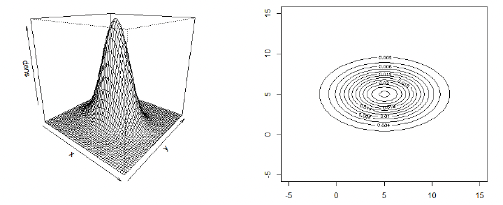
R Code for displaying density
1
2
3
4
5
6
7
8
9
10
11
12
13
14
15
16
17
18
19
20
21
# creates an appropriate grid
x1 <- seq(-5,15, length=51)  # 51 is an arbitrary grid size
x2 <- seq(-5,15, length=51)
dens <- matrix(0,51,51)

# defines mu and Sigma
mu <- c(5,5)
# 协方差矩阵(对角线元素非零,表示无相关)
Sigma <- matrix(c(9,0,0,4), byrow=TRUE, ncol=2)

# fills grid with density values
require(mvtnorm)
for (i in 1:51) {
  for (j in 1:51) {
    dens[i,j] <- dmvnorm(x=c(x1[i],x2[j]), mean=mu, sigma=Sigma)
  }
}
# 3D 透视图
persp(x1, x2, dens, theta=40, phi=20)  # draws the density in 3D
# 2D 等高线图
contour(x1, x2, dens)  # draws contour plots in 2D
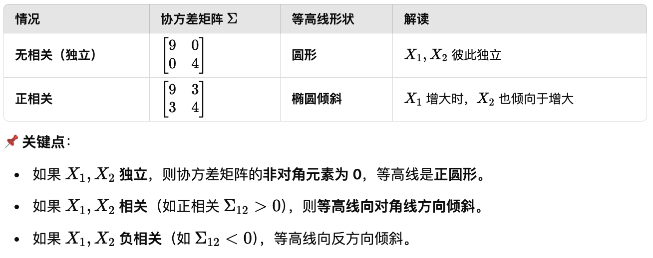
Some observations (based on the example from the last two slides):
- From the marginalization property, we can conclude that $X_1 \sim N(5, 3^2)$ and $X_2 \sim N(5, 2^2)$;
- For the matrix $\Sigma$ used in the last two slides, all entries off the diagonal are zero. Statistically, the entries off the diagonal are the covariances between the two random variables $X_1$ and $X_2$. If these are 0, then $X_1$ and $X_2$ are uncorrelated. If $X$ is MVN with uncorrelated components $X_1$ and $X_2$, then these are also independent, i.e. $f(x_1, x_2) = f(x_1) \times f(x_2)$.
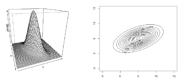
What happens if the two components are not uncorrelated? Assume now $Cov(X_1,X_2) = 3$, that is
\[\Sigma = \begin{pmatrix} 3^2 & 3 \\ 3 & 2^2 \end{pmatrix}\]The only actual difference to the previous code is
1
Sigma <- matrix(c(9,3,3,4), byrow=TRUE, ncol=2)
but for aesthetic reasons we slightly change the graphical parameters:
1
2
persp(x1, x2, dens, theta=40, phi=20)
contour(x1, x2, dens, nlevels=20)
Quick reminder: Variance matrix needs to be valid
Can we choose ‘anything’ for Σ?
No! It needs to be symmetric and positive definite or the density cannot be normalized. Check the latter via
1
2
eigen(Sigma)$values
## [1] 10.405125 2.594875
$\Sigma$ is positive definite if and only if all eigenvalues are positive.
Sometimes attributes operate on very different scales (for instance, kg, meters, etc.), which could distort the dissimilarities. This can be mitigated by defining appropriate weights. Common choices are
有时属性在非常不同的尺度上运作(例如,千克,米等),这可能会扭曲不同之间的差异。可以通过定义适当的权重来减轻这种情况
- 使用平均不相似度加权 (i) $w_j = \frac{1}{\bar{d}_j}$, where $\bar{d}_j$ is the mean over all $n^2$ pairwise dissimilarities over all $n$ observations (gives all attributes equal influence) [H1 Sec 14.3.3].
让所有属性在计算不相似度时具有相等的影响力。
- 使用方差归一化 (ii) $w_j = \frac{1}{\sigma_j^2}$, where $\sigma_j$ is the (known or estimated) standard deviation of the $j$th attribute (scales all attributes to unit variance).
- 将所有变量的方差缩放到相同的范围(单位方差)。
Mahalanobis distances 马哈拉诺比斯距离
The dissimilarities created in (ii) can be written as
\(D(x_i, x_i') = \sum_{j=1}^{p} \frac{1}{\sigma_j^2}(x_{ij} - x_{ij'})^2 = (x_i - x_i')^T \begin{pmatrix} \sigma_1^{-2} \\ & \ddots & \\ & & \sigma_p^{-2} \end{pmatrix} (x_i - x_i')\)
- 这是一种归一化的欧几里得距离,考虑了变量的尺度(使用方差归一化)。
- 仍然没有考虑变量间的相关性(只考虑了个体变量的方差)。
广义马哈拉诺比斯距离 This can be generalized by replacing the diagonal matrix by the inverse of a full variance matrix $\Sigma$ (again, known or estimated), yielding what is known as the (squared) Mahalanobis distance:
\[D_M(x_i, x_i') = (x_i - x_i')^T \Sigma^{-1}(x_i - x_i')\]Have we seen this dissimilarity before? Yes, in MVN density!
Note that we can write the $N(\mu, \Sigma)$ density function as
\[f(x) = \frac{1}{(2\pi)^{p/2}|\Sigma|^{1/2}} \exp \left\{ -\frac{1}{2} D(x, \mu) \right\},\]therefore points with equal Mahalanobis distance to the mean lie on the same contour of the respective Gaussian distribution.
An interesting property of Mahalanobis distances to the mean is that, when considered as a random variable,
\[D_M(X, \mu) \approx \chi^2(p)\]where $\chi^2(p)$ denotes a $\chi^2$ distribution with $p$ degrees of freedom.
This result can be used for outlier detection and testing multivariate normality.
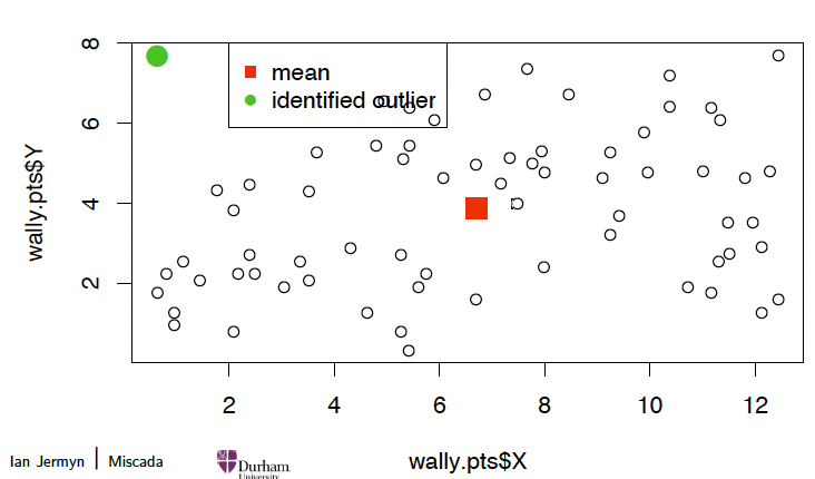
Outlier detection 异常值检测
For instance, for Wally’s data, compute all squared Mahalanobis distances and compare with the 2.5% tail quantile of χ²(2):
1
2
3
4
5
6
7
8
9
10
11
12
# 计算均值向量和协方差矩阵
wally.m <colMeans(wally.pts[,c("X","Y")])
wally.S <var(wally.pts[,c("X","Y")])

# 计算马哈拉诺比斯距离
wally.Mdist <mahalanobis(wally.pts[,c("X","Y")], center=wally.m, cov=wally.S)

# 检测异常值(2.5% 分位数)
detect <which(wally.Mdist > qchisq(0.975, 2))
detect  # 输出异常值索引

## [1] 1
1
2
3
4
5
6
7
plot(wally.pts$X, wally.pts$Y)  # 绘制所有数据点
points(wally.m[1], wally.m[2], pch=15, cex=2, col=2)  # 画出均值点
points(wally.pts$X[detect], wally.pts$Y[detect], pch=16, col=3, cex=2)  # 标记异常值

# 添加图例
legend(2,8, pch=c(15,16), col=c(2,3), legend=c("mean", "identified outlier"))
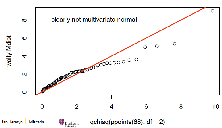
Checking multivariate normality 多元正态性检验
Compare to data generated from a MVN:
1
2
3
4
5
6
7
8
9
10
11
12
13
14
require(mvtnorm)

# 生成 300 个样本
mu <c(5,5)
Sigma <matrix(c(9,0,0,4), byrow=TRUE, ncol=2)
Z <rmvnorm(300, mean=mu, sigma=Sigma)

# 计算马哈拉诺比斯距离
Z.Mdist <mahalanobis(Z, mu, Sigma)

# 绘制 QQ 图
qqplot(qchisq(ppoints(300), df=2), Z.Mdist)
abline(a=0,b=1, col=2, lwd=2)
text(3,10,"clearly multivariate normal")
# Practical 1
In the first lab session (fetch Practical 1 on Jupyter), we will:
- carry out some simple exploratory data analysis of a four-dimensional, oceanographic data set;
- apply k-means to this data set; identify the cluster centres and visualize the clusters;
- experiment with different settings of k-means and different numbers of clusters;
- search for outliers and check for multivariate normality of this data set.